稀疏模型：起源、重要性以及LLM的前沿与未来

Overview

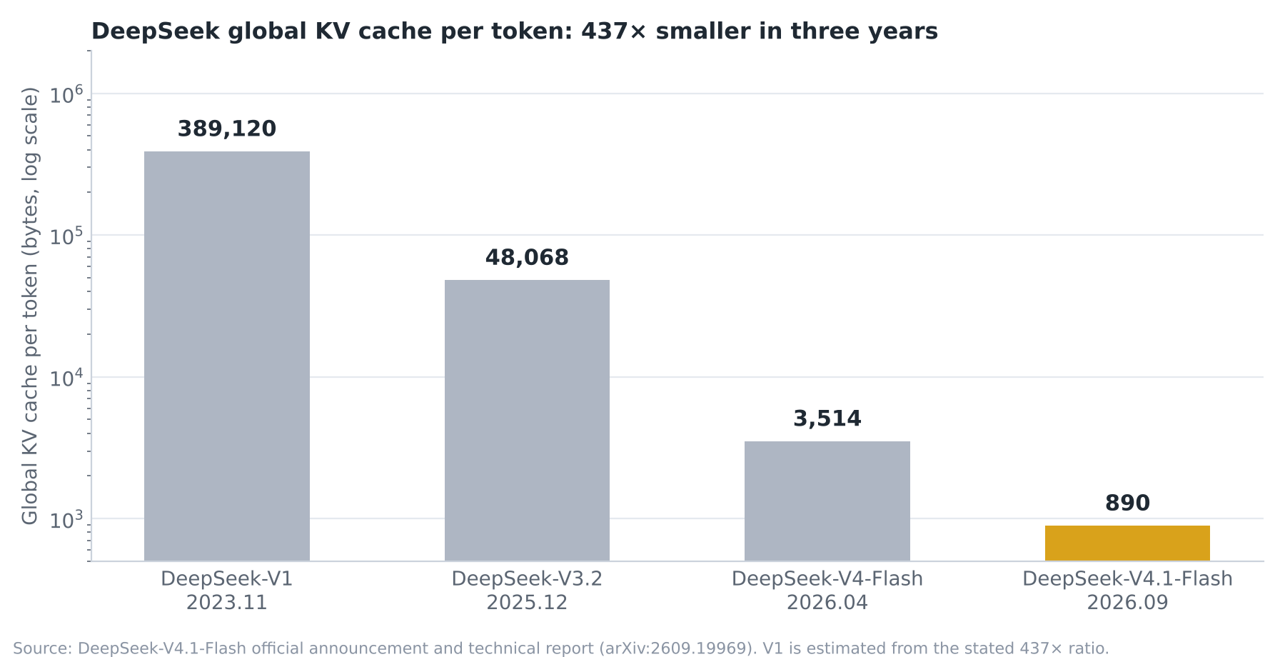
As of 2026, sparsity is no longer an optional efficiency trick. It is the default architectural constraint of frontier large models, and it decides both what a large model costs to run and how accurately a long-document agent can read. The most direct evidence is DeepSeek-V4.1-Flash, released on September 10, 2026. Its backbone has 552B parameters, yet it activates only 8B per token during prefill and 16B during decode, and the global KV cache resident in GPU memory has been compressed to 890 bytes per token, 1/437 of DeepSeek-V1’s (official DeepSeek announcement, technical report arXiv:2609.19969).

Three key takeaways

• The lineage of sparsity is continuous. From Barlow’s and Olshausen–Field’s “sparse coding in the brain,” through the “computable sparsity” of wavelets, LASSO, and compressed sensing, to the “sparsity as architecture” of MoE, sparse attention, and conditional memory, the same prior sits underneath: only a very few components truly matter. What the three successes share is that their sparsity pattern fit the hardware. Unstructured weight pruning lost not because of theory but because of hardware.

• Why now. Scaling ran into inference cost and the memory wall, and long-context agents turned the KV cache and prefill into the dominant costs. Sparsity’s role therefore widened from “saving compute” to “saving memory, bandwidth, and storage.” Mainstream MoE in 2024 activated roughly 25% of its parameters per token (Mixtral); by 2026 the figure has fallen to 1.5%–4.5% (DeepSeek-V4.1, Kimi K3, Qwen3.5).

• Sparsity is no panacea. The largest evaluation of sparse attention to date (Nawrot et al., Findings of ACL 2026) showed that nearly every sparse configuration suffers a large performance drop on at least one task. In interpretability, sparse autoencoders (SAEs) ran into systematic negative results in 2025. Model selection must be based not on average scores but on the tasks that are hardest for your own business.

Two threads that run through this survey

• The five kinds of sparsity: activation sparsity, weight sparsity, structured sparsity, conditional computation (MoE), and attention sparsity. The debate over “whether sparsity helps” cannot even begin until one specifies which kind.

• The three operators: soft thresholding (the proximal operator of L1), hard thresholding (L0), and top-k projection (projection onto the L0 ball). From wavelet denoising in 1994 to MoE routing in 2026, the step that “produces zeros” is nothing more than one of these three operators applied to a different object. Almost every modern large model uses the third, because it fixes the compute per token exactly and aligns with the parallel granularity of the hardware.

Five terms that recur throughout

Term	In a nutshell
Token	The smallest unit of text a model processes: a word, or part of one. “How many parameters are activated per token” means how much compute is spent each time a little more text is emitted
Parameters and activated parameters	Parameters are all the numbers a model stores (how much it knows). Activated parameters are the part actually used in computation when processing one token (what it costs to run). Sparsification means decoupling the two
Basis and coordinates	A set of “building blocks.” Data can be written as a weighted sum of them, and the weights are the coordinates. Change the blocks and the coordinate system changes: the data stays the same, but the values you read off change
Norms	L2 is length, L1 is the sum of the absolute values of the components, and L0 is the number of nonzero entries. Sparse means a small L0
FLOPs and memory bandwidth	Compute throughput is the number of multiply–accumulate operations per second; bandwidth is the number of bytes that can be moved out of GPU memory per second. In the decode stage of modern large models, the bottleneck is usually the latter

A note on terminology: This survey uses “sparse” strictly to mean “most of the elements are zero.” “Low rank” means “no element is zero, but there are few degrees of freedom” (MLA, LoRA, and so on). The two are often confused; this survey keeps them consistently distinct.

How to read this survey

This survey proceeds chronologically, and in each era it answers the same four questions. What were the background and the bottleneck at the time? By what mechanism did sparsity appear? What did it solve, and at what cost? How does it relate to today’s large models? The section “Prehistory” asks why the world is sparse; “The Classical Era” shows how mathematics turned that into a tool; and “The Neural Network Era” explains why pruning lost once sparsity entered neural networks. The central section, “The Present,” discusses why large models went all in on sparsification in 2023–2026 and systematically compares each lab’s approach. “Where Sparsity Meets Deep Learning” covers the fusion of sparsity and deep learning in imaging and signal processing, and the sections “Applications,” “Benefits and Costs,” “The Future,” and “What This Means for Us” take up applications, costs, the future, and what all of this means for us. The appendices collect a timeline, data, anecdotes, and references.

Prehistory: Why the World Itself Is Sparse

Sparsity is not a property of data alone; it is a property of “data plus the way we describe it.” The world becomes sparse under the right basis, and the history of science is in part the history of searching for that basis. This section lays out three kinds of empirical evidence and one intellectual wellspring, and then marks their limits.

Philosophy and information theory: intuition and framework, not technical origins

Occam’s razor is a philosophical principle that favors simplicity; it is not the technical starting point of sparse models. Shannon (1948) quantified “redundancy”: whatever part of a code length exceeds the entropy of the source is compressible redundancy, and a sparse representation is, at heart, a basis that brings that redundancy to the surface. Kolmogorov complexity (1960s) offered the ideal of “the shortest description,” but it is uncomputable; Rissanen’s MDL (1978) turned it into a practical criterion for model selection. A sparse model can be read as a special case of MDL: description length ≈ number of nonzeros × the coding cost per coefficient. These ideas should be written up as the “intellectual prehistory,” not as the “inventors of sparse models.”

Three kinds of evidence from nature

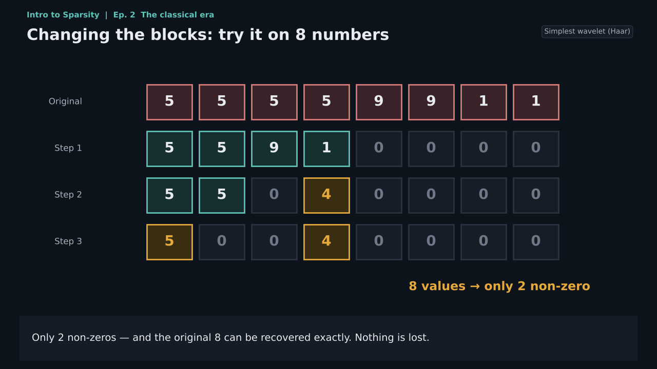
Natural images. The power spectrum of natural images approximately follows a 1/f² power law and exhibits approximate scale invariance (Field 1987; Ruderman & Bialek 1994; for a review, Simoncelli & Olshausen 2001). In a local, band-pass basis such as wavelets, the coefficients of natural images are heavy-tailed: most are close to zero, and only a few, at the edges, are large. Nonlinear approximation theory (DeVore 1998; Donoho 1993) proved that for piecewise smooth signals, the error of the best n-term approximation in a wavelet basis decays faster than in any fixed linear basis. This is the theoretical foundation of both JPEG2000 and compressed sensing, and the Haar example in Figure 3 is its smallest demonstration.

Language. Word frequencies follow Zipf’s law: a handful of words account for most occurrences, and the tail is extremely long. Bag-of-words and TF-IDF representations are therefore extremely sparse. The same statistics explain why the load on MoE experts is inherently skewed, and why DeepSeek uses an N-gram lookup table as conditional memory (Engram).

The brain. Barlow (1961) proposed the redundancy reduction hypothesis: the purpose of a sensory system is to strip out redundancy and build statistically independent representations. This is the neuroscientific source of sparse coding. Attwell & Laughlin (2001) worked out the energy budget of gray matter, and from it Lennie (2003, Current Biology 13:493–497) estimated that, because a single spike is so expensive, “the number of neurons that can be substantially active at the same time is probably severely limited to less than 1%.”

One correction is unavoidable here. The widely repeated claim that “the brain uses only 1–4% of its neurons” is a secondhand citation. When Glorot, Bordes, and Bengio (2011) cited Lennie, they wrote “1–4%,” and the figure has been reprinted ever since. Lennie’s original says “possibly fewer than 1%,” and even that is an estimated upper bound derived from energy constraints, not a measurement. Sparsity means “the fraction firing strongly at any one time is low”; it does not mean “most of the brain is idle.”

Limits and counterexamples

Sparse is not low rank. Sparse means few nonzero coefficients under some basis or dictionary (measured by L0/L1). Low rank means few singular values in a matrix (measured by rank or the nuclear norm). LoRA and MLA are low-rank; MoE, top-k attention, and SAEs are sparse. A truncated SVD yields a low-rank matrix; the only thing sparse about it is its singular-value spectrum.

The world is not always sparse. Robust PCA (Candès, Li, Ma & Wright 2011) decomposes data into “low-rank plus sparse” and showed that real data often has both: in video, the background is low-rank and the foreground is sparse. Signals dominated by texture or noise are not sparse in the commonly used bases. Feature superposition in the residual stream of an LLM means the representation is dense at the level of individual neurons and becomes sparse only under an overcomplete dictionary. That is the starting point of the SAE discussion in “The Present” (the section “Sparsity in interpretability”).

Summary of this section. Sparsity is a falsifiable prior, not a universal truth. It has been confirmed again and again in natural images, language, and neural activity, so it is worth “betting on.” But before placing the bet, one question must always be asked: sparse under which basis?

The three kinds of evidence in detail: why exactly these statistical laws

Where does the 1/f spectrum of natural images come from? There are two complementary explanations. The first is scale invariance. The sizes of objects in a natural scene span many orders of magnitude, and the statistics of an image do not change whether you zoom in or out; mathematically, that forces the power spectrum into a power law. The second is the occlusion model. A scene consists of objects overlapping one another front to back; edges produce discontinuities, and discontinuities appear in the frequency domain as a slowly decaying high-frequency tail. Both explanations arrive at the same conclusion: natural images are neither “random noise” nor “smooth everywhere,” but “wide flat regions plus a few edges.” This is precisely the structure a wavelet basis handles best. Field (1987) went further and pointed out that if the bandwidth of the receptive fields of simple cells in visual cortex matches these statistics, each cell’s response to natural images will be heavy-tailed: barely responding most of the time, firing strongly now and then. This is the original meaning of the term “sparse coding” in neuroscience.

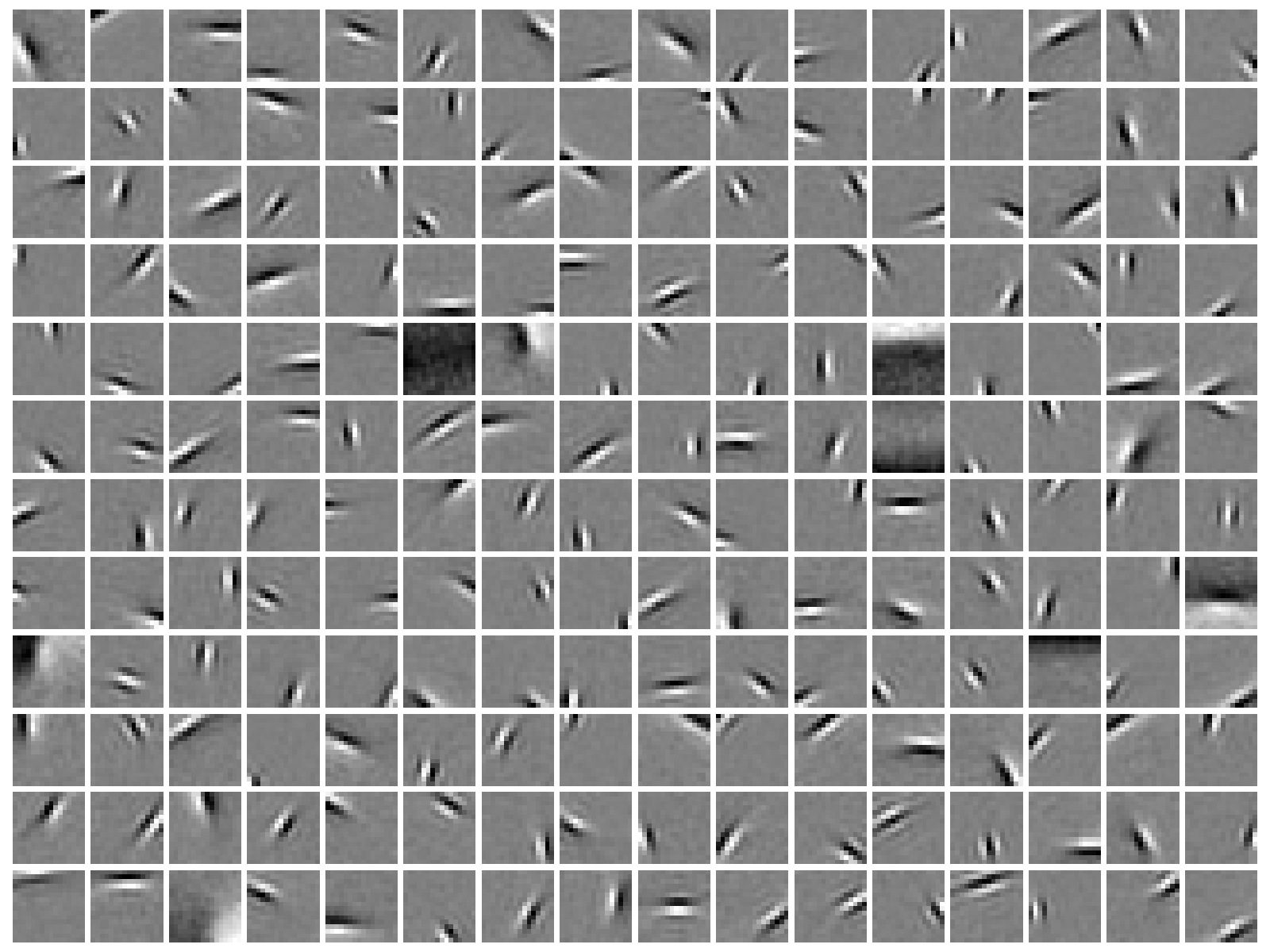
Why is the Olshausen and Field experiment so convincing? The 1996 experiment placed only two constraints on the algorithm: reconstruct patches of natural images with a set of linear basis functions, and make the coefficients as sparse as possible. There was no prior knowledge about the brain at all. Yet the learned basis functions came out local, oriented, and band-pass, and closely matched the receptive fields of V1 simple cells in cats and monkeys. The force of the result lies in its direction: it was not that “an algorithm was built by taking inspiration from the brain,” but that “the sparsity principle independently predicted the structure of the brain.” Later, Hromádka, DeWeese, and Zador (2008) recorded highly sparse firing patterns in the auditory cortex of awake rats, and Quian Quiroga et al. (2005) discovered “concept cells” in the human hippocampus that respond selectively to particular people or landmarks. Both are taken as evidence for the sparse coding hypothesis. There is dissent. Spanne and Jörntell (2015), among others, argue that strict sparse coding is not universal in cortex and that the degree of sparsity depends on brain region and task. It should therefore be written up as a “widely supported hypothesis,” not as settled doctrine.

Why does energy force sparsity? The human brain is about 2% of body weight but consumes about 20% of resting metabolism, roughly 20 watts. Attwell and Laughlin (2001) estimated that most of the energy in gray matter goes to synaptic transmission and action potentials. Lennie (2003) worked backward from there: if a single spike costs this much, the cortex cannot afford to have a large fraction of its neurons firing at high rates simultaneously. Because the argument is an “upper bound under a budget constraint,” it yields an estimate, “probably fewer than 1%,” rather than a measurement. Its significance lies in the logic, not the specific number. In a system with limited energy or bandwidth, sparsity is not an option but a necessity. The same logic is replayed in “The Neural Network Era” as the “memory wall” on GPUs.

Zipf’s law and the long tail in language. Zipf (1935) observed that a word’s frequency is roughly inversely proportional to its rank: the second most common word appears about half as often as the first, the tenth about one-tenth as often. Mandelbrot later gave a corrected form. The direct consequence is that any text uses only a tiny fraction of the vocabulary, and most words appear only once or twice. In the era of statistical language models, this showed up as extremely sparse n-gram frequency matrices and as the smoothing problem of “zero probabilities” (Good–Turing, Kneser–Ney). In the era of large models it has returned in two forms. One is the inherently skewed routing load in MoE: popular experts take on most of the tokens, so a load-balancing mechanism has to intervene. The other is DeepSeek’s Engram, which brings the N-gram lookup table back into a frontier architecture, sending frequent patterns down a cheap lookup path and leaving only what genuinely needs reasoning to the expensive Transformer layers.

Sparsity in physics and engineering

Sparsity has a longer history in engineering than in machine learning. In scientific computing, the coefficient matrices of the finite element method and of power-flow equations are inherently sparse: each node couples only to its neighbors. Tinney and Walker (1967), solving power systems, proposed an optimal ordering that reduces “fill-in” during Gaussian elimination. That was the starting point of sparse direct methods. Rose (1972) then described the elimination process in graph-theoretic terms, Gilbert and others developed sparse LU factorization, and sparse linear algebra became a field of its own. In seismic exploration, the subsurface reflectivity series is modeled as a sparse train of spikes, and the deconvolution problem can be solved with L1 regularization, 20 years ahead of compressed sensing. In radar and array signal processing, targets are sparsely distributed in the space of angle, range, and velocity, and sparse recovery is used for super-resolution estimation.

What these fields share is that the sparsity pattern comes from physical structure (adjacency, reflections, the number of targets), which makes it predictable and exploitable. This is continuous with wavelets in “The Classical Era” (where the structure comes from piecewise smoothness) and with MoE in “The Present” (where the structure comes from expert blocks), and it also explains why unstructured weight sparsity loses in “The Neural Network Era”: its zeros have no physical structure, and the hardware cannot exploit them.

Mirrors in social phenomena, and the limits of the idea

Pareto’s 80/20 rule, Anderson’s long tail, and the factor-analysis tradition that “a few important variables explain most of the variance” are all mirrors of the sparsity prior in the social sciences. What they show is that sparsity is an assumption about the structure of the world, not a theorem. Statisticians such as Gelman have questioned the “bet on sparsity”: in many problems in social science, they argue, the true effects are dense and small, and sparse methods systematically miss them. The same criticism applies to machine learning. Features in an LLM’s residual stream are stored densely through superposition, and sparsity emerges only once we switch to an overcomplete dictionary. The position of this survey is therefore as follows. Sparsity has been confirmed repeatedly across vast amounts of natural data, so it is a prior worth betting on first. But every time we place the bet, we must answer “sparse under which basis?” and be ready to let go if the evidence does not support it.

The Classical Era (1960s–2014): How Sparsity Became a Computable Tool

The sparse methods that succeeded in the classical era share one trait: their sparsity patterns were structured and predictable, so they could be absorbed into hardware and industry standards. This foreshadows the “failure” described in “The Neural Network Era.” The table below organizes the milestones around three questions: why each appeared when it did, what the bottleneck of the day was, and what it solved.

Milestone	Why it appeared then	The bottleneck of the day	What it solved
Direct methods for sparse matrices (Tinney & Walker 1967)	Power grids were scaling up; memory was measured in KB	Dense elimination is O(n³) and does not fit in memory	Store only the nonzero entries; reduce fill-in with optimal ordering
Wavelets (Daubechies 1988; Mallat 1989)	The Fourier basis is not sparse for edges	Edge energy spreads across the frequency domain	Piecewise smooth signals become sparse in the wavelet domain
Matching Pursuit (Mallat & Zhang 1993)	The arrival of overcomplete dictionaries	Representations are not unique	Greedy atom selection
Wavelet thresholding denoising (Donoho & Johnstone 1994)	Coefficients are sparse; noise is uniform	Linear filters blur edges too	Soft thresholding = the proximal operator of L1; near minimax optimal
Breiman’s garrote 1995 → LASSO (Tibshirani 1996)	High-dimensional data, p ≫ n	Least squares is ill-posed; subset selection is unstable	Shrinkage and variable selection at once
Basis Pursuit (Chen, Donoho & Saunders 1998)	Convex optimization had matured	L0 is NP-hard	Convex relaxation via L1
Nonlinear approximation (DeVore 1998)	An explanation was needed for why keeping the k largest entries is optimal	Linear approximation converges slowly	The theory of best n-term approximation
JPEG (1992) / JPEG2000 (2000)	Digital images went mainstream	Bandwidth and storage	Sparse transform + quantization + entropy coding
LARS (Efron et al. 2004); Elastic Net (Zou & Hastie 2005)	LASSO needed an efficient path algorithm	Slow to solve; unstable with correlated variables	Compute the entire regularization path at once; L1 + L2
Compressed sensing (Candès–Romberg–Tao 2006; Donoho 2006)	Sparse theory met random matrix theory	Sampling was bound by Nyquist	Recovery from m ≳ k·log(n/k) measurements under the RIP condition
K-SVD (Aharon, Elad & Bruckstein 2006)	Learnable dictionaries were needed	Fixed wavelets do not fit specific data	Alternate sparse coding with dictionary updates
Donoho–Tanner phase transition (2009)	A characterization of when L1 succeeds was needed	Theoretical upper bounds were too loose	A sharp phase transition in the (m/n, k/m) plane
Sparse coding (Olshausen & Field 1996); fast algorithms (Lee, Battle, Raina & Ng 2007)	A response to Barlow’s hypothesis	Why are V1 receptive fields Gabor-like?	Sparse dictionaries reproduce V1 receptive fields
The cat-face neuron (Le et al. 2012)	The arrival of distributed training	Do higher-order features emerge without supervision?	See below
Optimal singular-value hard thresholding (Gavish & Donoho 2014)	Low-rank denoising needed a principled threshold	Truncation rank was chosen by rule of thumb	For square matrices, (4/√3)√n·σ when σ is known; 2.858 × median when unknown

The “bet on sparsity” principle in statistics

Hastie, Tibshirani, and Friedman advocated the “bet on sparsity” principle in The Elements of Statistical Learning. If the true model is sparse, L1 can find it. If it is not sparse, no method works well. Therefore, bet on sparsity. High-dimensional statistics then quantified the exact price. To recover a k-sparse vector in p dimensions, n ≳ k·log p samples suffice (Wainwright 2009). The corresponding result in compressed sensing is m ≳ C·k·log(n/k) random measurements, with exact recovery by L1 whenever the RIP constant satisfies δ₂ₖ < √2−1 ≈ 0.414 (Candès 2008).

Three real-world cases (figures verified)

CS-MRI. Lustig, Donoho, and Pauly (2007) laid the foundations of compressed-sensing MRI. The clinical figures need to be quoted precisely. Sartoretti et al. (2019, PLoS ONE 14(4): e0214887) report that in routine clinical practice the mean scan time fell by 20.2%, examination duration fell by 16%, acquisition time for the applicable sequences fell by 23%–43%, and the number of examinations over the same period rose by 27% (primary source). Vranic et al. (2019, AJNR 40(1):92–98) report reductions of 25% and 35% for brain FLAIR and GRE sequences, respectively. The oft-cited “30%–60% speedup” has no backing in the primary sources.

Black hole imaging (EHT). SMILI, one of the three imaging pipelines behind the first image of M87* in 2019, descends from the sparse modeling (L1 + TV regularization) of Honma et al. (2014) and Akiyama et al. (2017). Another pipeline, CHIRP (Bouman et al. 2016), uses patch priors rather than pure compressed sensing, so the press story that “a single researcher photographed a black hole with compressed sensing” is a simplification.

The cat-face neuron. Le et al. (2012, ICML, arXiv:1112.6209) trained a nine-layer, locally connected sparse autoencoder with about one billion connections on 10 million YouTube frames, “on 1,000 machines (16,000 cores) for three days.” Without supervision, single neurons emerged that responded selectively to human faces and cat faces, and downstream on ImageNet the model reached 15.8% accuracy, a relative improvement of 70% over the previous best. This “sparse coding → unsupervised features” lineage faded after 2012 under pressure from supervised CNNs, then returned in 2023 as Anthropic’s SAEs.

A parallel line: low rank

Truncated SVD (the Eckart–Young–Mirsky theorem) is the best approximation among all matrices of rank at most k, and Gavish & Donoho (2014, IEEE T-IT 60(8):5040–5053) gave the optimal hard threshold for denoising. This is structurally isomorphic to wavelet thresholding denoising. Both follow “change basis → threshold → transform back”; the only difference is that the wavelet basis is fixed while the SVD basis is computed from the data. In the former, the signal stays sparse after thresholding; in the latter, the truncated matrix is low-rank but dense. This lineage returns to large models in “The Present,” in the form of MLA and LoRA.

Step by step: why each advance happened when it did

From Fourier to wavelets (1980s). The Fourier basis decomposes a signal into global sinusoids. That is efficient for stationary signals but extremely wasteful for edges and transients: representing a single step requires infinitely many frequency components, and the energy spreads across the frequency domain. Engineering already had workarounds, such as the Gabor transform and the short-time Fourier transform, but it lacked a unified mathematical framework. Mallat (1989) formalized multiresolution analysis, and Daubechies (1988) constructed orthogonal wavelets with compact support, making it possible to satisfy all three of locality, multiscale structure, and orthogonality at once. Each wavelet basis function is nonzero only over a finite range, and it recurs at every scale. A piecewise smooth signal therefore produces large coefficients only at edge locations and at a few scales, with everything else close to zero. DeVore (1998) and Donoho (1993) proved that this is no empirical accident: for the class of piecewise smooth functions, no fixed linear basis can match the error decay rate of the best n-term nonlinear approximation in a wavelet basis. JPEG2000 (2000) turned this theory into a standard, replacing JPEG’s DCT with wavelets and greatly reducing blocking artifacts at the same bit rate.

From least squares to LASSO (1990s). Statistics faced a different kind of sparsity: not whether the coefficients are sparse in some basis, but “which explanatory variables actually matter.” The classical approach was subset selection (stepwise regression, AIC/BIC), but it is a combinatorial search and extremely unstable under small perturbations of the data. Breiman (1995) proposed the non-negative garrote, recasting variable selection as a continuous shrinkage problem. Inspired by it, Tibshirani (1996) proposed the LASSO: least squares with an L1 penalty. The geometry of L1 determines its behavior. The constraint region is a diamond with corners, the optimum tends to land on a corner, and each corner corresponds to a point where some coefficients are exactly zero. This is the mechanism by which “shrinkage and selection happen at once.” The LASSO’s algorithmic bottleneck was removed in 2004 by LARS (Efron, Hastie, Johnstone, and Tibshirani), which made it possible to compute the entire regularization path in one pass. In 2005, Zou and Hastie’s Elastic Net handled groups of strongly correlated variables with L1 + L2. High-dimensional statistics then supplied the theoretical guarantees. Wainwright (2009) proved that n ≳ k·log p samples suffice to recover k nonzero coefficients in p dimensions, and Bickel, Ritov, and Tsybakov (2009) established oracle inequalities for the LASSO and the Dantzig selector.

An independent discovery in signal processing (1993–1998). At almost the same time, signal processing started from “overcomplete dictionaries” and arrived at the same L1. Matching Pursuit (Mallat and Zhang 1993) greedily selects the atom most correlated with the residual, and Basis Pursuit (Chen, Donoho, and Saunders 1998) relaxed the NP-hard L0 problem of “finding the sparsest representation” into an L1 linear program. The LASSO and Basis Pursuit are mathematically two parameterizations of the same problem, yet they emerged from two communities that barely interacted. This is the first instance of the idea of sparsity “converging from multiple sources.”

Denoising: the first time sparsity directly created value (1994). Donoho and Johnstone’s wavelet thresholding denoising turned the theory above into a three-step procedure. Move to the wavelet domain with an orthogonal transform. Apply soft thresholding S_λ(w)=sign(w)·max(|w|−λ,0) to the coefficients, with threshold λ=σ√(2 log n). Return to the signal domain with the inverse transform. The key to why this works is that an orthogonal transform preserves the statistical properties of white noise. In the wavelet domain, the noise remains independent Gaussian noise of equal variance, spread evenly over all coefficients, while the signal’s energy concentrates in a few large coefficients, so it suffices to discard the small ones. The soft thresholding operator is exactly the proximal operator of the L1 penalty, which is why denoising, the LASSO, and later ISTA/FISTA (Beck and Teboulle 2009) and LISTA (Gregor and LeCun 2010, the starting point of algorithm unrolling) all share the same core operation.

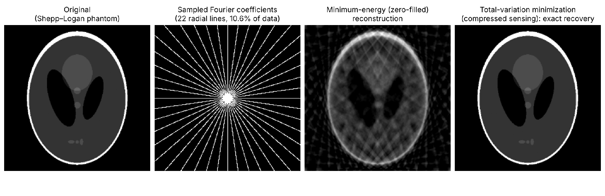
Compressed sensing: turning sparsity into “measure less, get more” (2004–2009). Every method so far searched for a sparse representation on the assumption that complete data was available. Candès, Romberg, and Tao (2006) and Donoho (2006) asked the reverse question: if a signal is known to be k-sparse in some basis, how many measurements are needed for exact recovery? The answer is m ≳ C·k·log(n/k) random linear measurements, far below the Nyquist rate. The condition is that the measurement matrix satisfy the restricted isometry property (RIP), that is, approximately preserve the length of every 2k-sparse vector. Candès (2008) gave the sufficient condition δ₂ₖ < √2−1 ≈ 0.414, and Donoho and Tanner (2009) used combinatorial geometry to characterize the sharp phase transition between success and failure of L1 recovery. The historical significance of compressed sensing is that it elevated sparsity from “a property of representations” to “a principle of sampling,” directly changing the design of imaging hardware. Lustig, Donoho, and Pauly (2007) brought it to MRI, trading random undersampling trajectories for shorter scan times. Duarte et al. (2008) built the single-pixel camera, and in radio astronomy the SMILI pipeline used L1 and total variation regularization for the EHT’s black hole imaging.

Dictionary learning and sparse coding: from fixed bases to learned bases (1996–2012). Wavelets are a fixed, human-designed basis, and not necessarily optimal for specific data. Olshausen and Field (1996) learned a dictionary from data and reproduced the receptive fields of V1. K-SVD (Aharon, Elad, and Bruckstein 2006) gave a practical algorithm that alternates sparse coding with atom-by-atom SVD updates. Lee, Battle, Raina, and Ng (2007) sped up L1 sparse coding and advanced “self-taught learning.” Le et al. (2012) stacked sparse autoencoders up to nine layers and one billion connections, learning cat-face-selective neurons without supervision from 10 million YouTube frames. After AlexNet in 2012, this lineage was overshadowed for a decade by supervised convolutional networks, but it left two things behind: a representational framework, “overcomplete dictionary + sparse coefficients,” and a conviction, “dictionaries can be learned from data.” When Anthropic decoded the internal features of large models with sparse autoencoders in 2023, it cited precisely Olshausen and Field, and a co-author of the companion paper was Olshausen himself.

Low rank: sparsity’s twin (1936–2014). Eckart and Young (1936) proved that the truncated SVD is the best low-rank approximation of a matrix. Low rank and sparsity are structurally isomorphic: both “concentrate energy in a few components and cut off the tail,” but they act on different objects. Sparsity cuts coordinates; low rank cuts directions. Gavish and Donoho (2014) gave the optimal hard threshold for low-rank denoising, echoing the universal threshold of wavelet denoising. Robust PCA (Candès et al. 2011) combined the two: data = low rank + sparse. This distinction becomes critically important in “The Present.” DeepSeek’s MLA is low-rank compression; DSA and CSA2 are the sparse attention. The two are often confused.

Summary: the three legacies the classical era left to deep learning

First, finding the right basis matters more than processing the data. The same image is dense in the pixel basis and sparse in the wavelet basis; the entire difference lies in how it is described. Second, only three operations create zeros: soft thresholding (L1), hard thresholding (L0), and keeping the k largest entries (projection onto the L0 ball). Third, only structured sparsity makes it into hardware and standards. Wavelet trees made it into JPEG2000, and random undersampling made it into MRI products. All three legacies reappear, each in a new guise, in “The Neural Network Era” and “The Present.”

The Neural Network Era (1990–2022): Sparsity’s Setback and Turning Point

Sparsity did not lose. Sparsity that did not fit the hardware lost. Unstructured weight pruning succeeded in theory and was defeated on the GPU. MoE made the unit of sparsity an entire expert block, and because the inside of each expert remained a dense matrix multiplication, it won the hardware lottery. This section explains why.

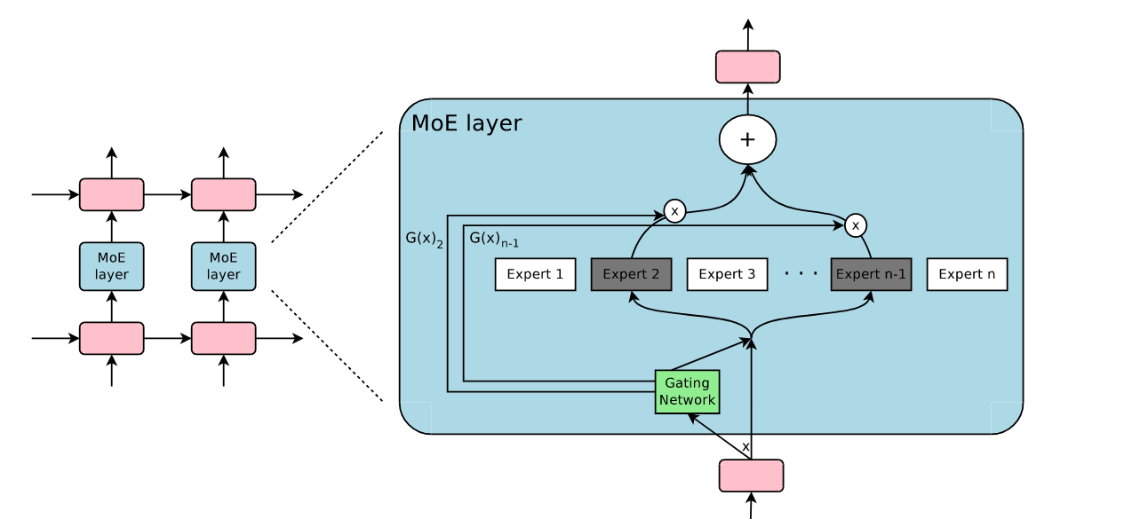
The pruning lineage and the “sparsity wall”

OBD (LeCun, Denker & Solla 1990) estimated the importance of each weight from second-order information, and OBS (Hassibi & Stork 1993) refined it with the full Hessian. Deep Compression (Han, Mao & Dally 2016) combined pruning, quantization, and Huffman coding to shrink AlexNet from 240 MB to 6.9 MB. The lottery ticket hypothesis (Frankle & Carbin 2019) showed that a dense network contains sparse subnetworks that, trained in isolation, reach the same accuracy. SparseGPT (Frantar & Alistarh 2023) and Wanda (Sun et al. 2023) showed that GPT-class models can be pruned to 50% sparsity in one shot with almost no loss of accuracy.

Once the LLM era arrived, however, this lineage hit a wall. The ELSA paper of October 2025 (arXiv:2510.01650) calls it the sparsity wall: existing methods “appear unable to exceed 50–60% sparsity without a substantial loss of accuracy.” ELSA claims that with ADMM, LLaMA-2-7B can be pruned to nearly 90%, but that claim is still being debated.

Activation sparsity: the real numbers behind ReLU

Glorot, Bordes, and Bengio (2011, AISTATS) is the primary source on activation sparsity, and its numbers deserve to be quoted precisely. Immediately after uniform initialization, about 50% of hidden units output exact zeros. After training, the average strict sparsity is 83.4% on MNIST, 72.0% on CIFAR10, 68.0% on NISTP, and 73.8% on NORB. The conclusion is that “the models that generalize best have sparsity between 50% and 80%,” and that sparsity can be enforced up to about 85% without hurting performance. The claim that “ReLU is 90% sparse” has no support in the original source.

One distinction is worth making in passing. Dropout is a random regularizer applied during training; at inference the network returns to being dense. Pruning deletes weights permanently. Both can be written as “applying a mask,” but the randomness of the mask, the stage at which it acts, and its purpose are entirely different.

Why unstructured weight sparsity lost in the GPU era

The hardware lottery. By Hooker’s definition (The Hardware Lottery, 2020/2021), a research idea wins because it fits the software and hardware available, not because it is the better idea. GPUs and TPUs are designed for dense, contiguous matrix multiplication. Unstructured sparsity brings in gather/scatter, breaks the tiled dataflow of GEMM, reduces on-chip cache reuse, and usually cannot use the tensor cores. Empirically, libraries such as cuSPARSE show a clear speedup only once sparsity exceeds roughly 90%; at 50% unstructured sparsity, almost no off-the-shelf kernel beats dense GEMM on a GPU.

2:4 structured sparsity. GPUs from Ampere onward support a pattern in which exactly two of every four weights are zero, and when the pattern is met the theoretical throughput doubles. But sparsity is capped at 50%, recovering accuracy requires retraining or fine-tuning, and end-to-end speedups rarely approach 2×, so in LLM deployment it has not spread as widely as quantization.

Why quantization won. Quantization reduces the number of bits per parameter but leaves the regularity of the matrix untouched, so every GPU benefits naturally. After GPTQ (2022) and AWQ (2023), MXFP4 became the native format of 2025–2026. gpt-oss stores its MoE weights (more than 90% of all parameters) in MXFP4 (4.25 bits per parameter), which is what lets the 120b model fit on a single 80 GB GPU. Kimi K3 does quantization-aware training with MXFP4 weights and MXFP8 activations, and the expert parameters of the DeepSeek-V4 series use FP4.

The memory wall. From the V100 to the B200, growth in peak compute far outstripped growth in memory bandwidth (order-of-magnitude figures based on published vendor specifications).

GPU	Dense BF16/FP16 compute	HBM bandwidth	Operations per byte (approx.)
V100 (2017)	~125 TFLOPS	0.9 TB/s	140
A100 (2020)	~312 TFLOPS	1.6–2.0 TB/s	155–195
H100 SXM (2022)	~989 TFLOPS	3.35 TB/s	295
B200 (2024)	~2.2 PFLOPS (~9 PFLOPS in FP4)	~8 TB/s	280 (~1,100 in FP4)

During decoding, every generated token requires the weights that take part in the computation to be moved out of GPU memory. At small batch sizes the arithmetic units sit mostly idle and the bottleneck becomes bandwidth. That is why “reducing the parameters and KV that must be read” is worth more than “reducing FLOPs.” MoE reduces the bytes of weights read per token; sparse attention and KV compression reduce the bytes in the cache. They are cutting exactly the most expensive line item.

The lineage of conditional computation (the turning point)

• 1991 Adaptive Mixtures of Local Experts by Jacobs, Jordan, Nowlan, and Hinton. It trained multiple expert networks together with a gating network, and the original motivation was to reduce interference between tasks. In 1994, Jordan & Jacobs extended it to hierarchical MoE.

• 2013 Bengio et al. proposed conditional computation and gradient estimation through stochastic neurons (STE). Eigen, Ranzato, and Sutskever made an early attempt at MoE in deep networks.

• 2017 Outrageously Large Neural Networks by Shazeer et al. (with Hinton and Dean as co-authors). It inserted sparsely gated MoE layers of up to 137B parameters between LSTM layers and achieved “greater than 1000x improvements in model capacity with only minor losses in computational efficiency.” Note that the original says greater than 1000x, and that 137B refers to the parameter count of the MoE layer.

• 2020–2022 GShard brought MoE into the Transformer and scaled it past 600B, and Switch Transformer (Fedus, Zoph & Shazeer 2021) reached one trillion parameters with top-1 routing. GLaM and ST-MoE tackled stability problems (router z-loss), and Expert Choice (2022) flipped the scheme so that experts choose tokens, which balanced the load naturally.

To put this section in one sentence: from 1991 to 2022 the idea of conditional computation did not change; what changed was that the hardware and the scale to match it finally arrived.

MoE from paper to product: the engineering problems solved in 2017–2022

Shazeer et al. (2017) showed that capacity could be expanded 1000-fold, but turning MoE into a dependable product took another five years and required solving four concrete problems.

How to learn the routing. The gate outputs s = Softmax(W_g·h), the top k experts are selected, and the layer’s output is y = h + Σ_{i∈T} s_i·FFN_i(h). The problem is that top-k is a discrete choice, so its derivative with respect to s is zero almost everywhere. Gradients reach only the gate weights of the selected experts, and experts that are not selected never get to learn. Shazeer’s solution was Noisy Top-k Gating, which adds learnable Gaussian noise to the logits so that the expert that would have ranked k+1 is occasionally chosen. The more general solutions come from the straight-through estimator (STE) of Bengio et al. (2013) and, later, Gumbel-Softmax.

How to balance the load. Routers have a rich-get-richer tendency. The more popular an expert, the more often it is chosen, the better it is trained, and the more likely it is to be chosen again, until a handful of experts carry all the traffic and the model degenerates into a small one (expert collapse). GShard and Switch Transformer introduced an auxiliary load-balancing loss L_bal = α·N·Σ f_i·P_i, where f_i is the fraction of tokens assigned to expert i and P_i is its average gate probability. ST-MoE (2022) went further and used router z-loss to keep the logits from exploding. These auxiliary losses work, but they disturb the gradients of the main language-modeling objective. In 2024, DeepSeek-V3 sidestepped the trade-off with a “bias that stays out of the gradient” (see “The Present”).

How to set capacity. In distributed training, the buffer size of each expert must be fixed in advance, and that is where the capacity factor comes in: capacity per expert = capacity_factor × (number of tokens / N). Tokens beyond capacity are dropped (token dropping) and pass through the residual connection alone. A large capacity factor wastes memory; a small one hurts quality. MegaBlocks (2023) escaped this dilemma by using block-sparse matrix multiplication to build “dropless” MoE.

How to survive the communication. Experts live on separate GPUs (expert parallelism), and each MoE layer requires two data-dependent all-to-all exchanges: tokens are sent to the GPU that holds the expert, and the results are collected back. This is the main communication bottleneck in MoE training, and it is also why MoE suits large, centralized deployments. From DeepSpeed-MoE and Tutel to DeepSeek’s DeepEP, every one of these systems optimizes this path.

Milestones: GShard (2020) brought MoE into the Transformer and scaled it past 600B; Switch Transformer (2021) reached one trillion parameters with top-1 routing and pretrained 4× faster than T5-XXL. GLaM (2021) had 1.2T total parameters and about 97B activated, and consumed roughly one third of the energy of GPT-3. Expert Choice (2022) reversed the direction, letting experts choose tokens, and balanced the load naturally.

Why MoE was still not mainstream before 2022

Even with these engineering solutions in hand, MoE in 2022 was still a “big-company toy” inside Google. There were three reasons. First, the cost pressure was not yet strong enough. In the GPT-3 era, dense models were still advancing rapidly, and inference cost was not the main constraint. Second, there was no open ecosystem. With no high-quality open-weight MoE, the community could neither reproduce nor improve on it. Third, fine-tuning was hard. Routing collapsed easily on small datasets, and adaptation to downstream tasks did not go as smoothly as for dense models.

All three conditions changed at once at the end of 2023. Mixtral 8x7B (2023-12) became the first high-quality open MoE; ChatGPT-scale traffic made inference cost the most pressing problem; and DeepSeekMoE (2024-01), with fine-grained experts and shared experts, pushed the cost efficiency of MoE to a new level. This is where “The Present” begins.

Summary

The three lineages of this section, namely pruning, activation sparsity, and conditional computation, met entirely different fates before 2022. Pruning succeeded in theory and lost on hardware. Activation sparsity (ReLU) was used everywhere and exploited almost nowhere. Conditional computation had everything in place and lacked only the economic pressure. Understanding these different fates explains why the winner after 2023 was MoE rather than weight pruning. Whether sparsity can be put to practical use is decided by whether its zeros have a structure the hardware can exploit.

The Present (2023–September 2026): Why LLMs Went All In on Sparsity

By 2026, the activation ratio per token of the most advanced open models had fallen to 1.5%–4.5%, and sparsity had spread from the FFN to attention, the KV cache, and the storage of knowledge itself. This section first lays out four pressures, then takes stock of each of the five kinds of sparsity in turn, and finally turns to a unifying theory and the economics.

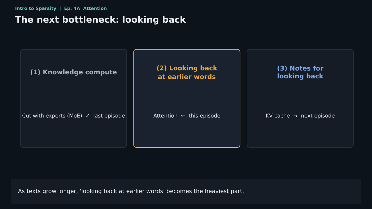
Why now: four pressures

• Scaling hit the cost wall. Total parameters reached the 1–3T range (DeepSeek-V4-Pro at 1.6T, Kimi K3 at 2.8T), and training and inference with dense models became unaffordable.

• Inference costs overtook training costs. In its inference-system overview of 2025-03-01, DeepSeek used large-scale expert parallelism spanning nodes to enlarge batches and raise GEMM efficiency. It shows that the economics of inference had become the single most important constraint on architecture design.

• Agents made workloads “input-centric.” The V4.1 technical report opens by stating that, with the spread of long-running agents, workloads are increasingly dominated by input, and enormous KV caches keep straining the capacity and transfer bandwidth of HBM and SSDs.

• Engineering ingenuity under export controls. DeepSeek-V3 was trained on 2,048 H800s, using roughly 2.788M GPU-hours in total. The H800 is the same chip as the H100, but its NVLink bandwidth was cut from 900 GB/s to 400 GB/s, and this directly gave rise to communication optimizations such as DeepEP.

Conditional computation: MoE becomes the default architecture

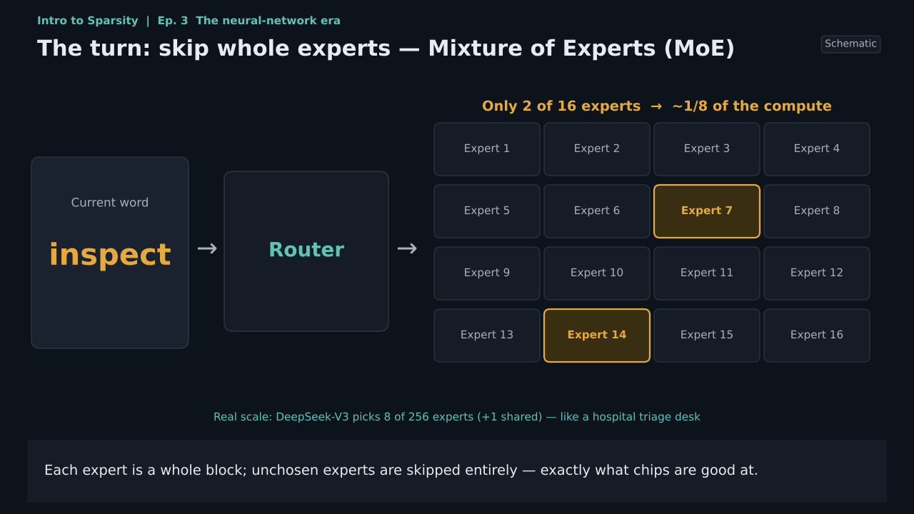
The evolution of the DeepSeek family (all from official technical reports, model cards, and API announcements):

Model	Date	Total parameters / activated per token	Expert configuration	Main sparsification techniques
DeepSeekMoE	2024-01	—	Fine-grained experts + shared experts	Splits experts finely, increasing the number of combinations exponentially
V2	2024-05	236B / 21B	2 shared + 160 routed	MLA: low-rank joint compression of KV (low-rank, not sparse)
V3	2024-12	671B / 37B	1 shared + 256 routed, 8 selected	Auxiliary-loss-free load balancing, multi-token prediction, FP8 training
V3.2	2025-09/12	671B / 37B	Same as above	DSA: Lightning Indexer + token-level top-k (k=2048) sparse attention
V4-Flash / V4-Pro	2026-04-24	284B/13B; 1.6T/49B	1 shared + 256 routed, 6 selected; 384 routed	Alternating Compressed Sparse Attention (CSA) and HCA; 1M context; FP4 experts
V4.1-Flash	2026-09-10	552B backbone + 196B Engram; prefill 8B / decode 16B	1 shared + 384 routed, 6 selected	CED, CSA2, Hierarchical Sparse Indexer, FP4 KV, Engram

The five design elements of V4.1-Flash (technical report):

• CED (Causal Encoder–Decoder). The 40 layers are split into a 20-layer encoder and a 20-layer decoder, and the decoder’s global KV is projected from the encoder’s final hidden states. Input tokens pass through the encoder only (8B activated), while output tokens pass through the decoder (16B). It is a direct answer to the fact that “agents read a lot and write a little.”

• The three modes of CSA2. Full generates its own global KV and builds an index. Reindex reuses the previous layer’s KV but recomputes the top-k. Reuse reuses even the top-k indices as they are. The great majority of layers are Reuse, which is to say that the great majority of layers “do not re-select tokens.”

• Hierarchical Sparse Indexer. The first Full layer of the decoder builds a candidate pool, and subsequent layers select only from within it. The cost of index computation in deep layers is decoupled from the context length.

• The KV numbers. Global KV is 890 bytes per token, about 1/4 of V4-Flash and 1/437 of V1. Persisted KV is about 1/8 of V4-Flash. Even when the context is widened from 4K to 1M (256×), the decode FLOPs per token grow by only about 1/4. Sparse attention is trained at 64K from the start, with no dense pre-warmup.

• Engram conditional memory. An N-gram hash table of roughly 196B parameters, accessed sparsely through per-token lookups, which can be placed in host memory and prefetched. It is not activated for every token.

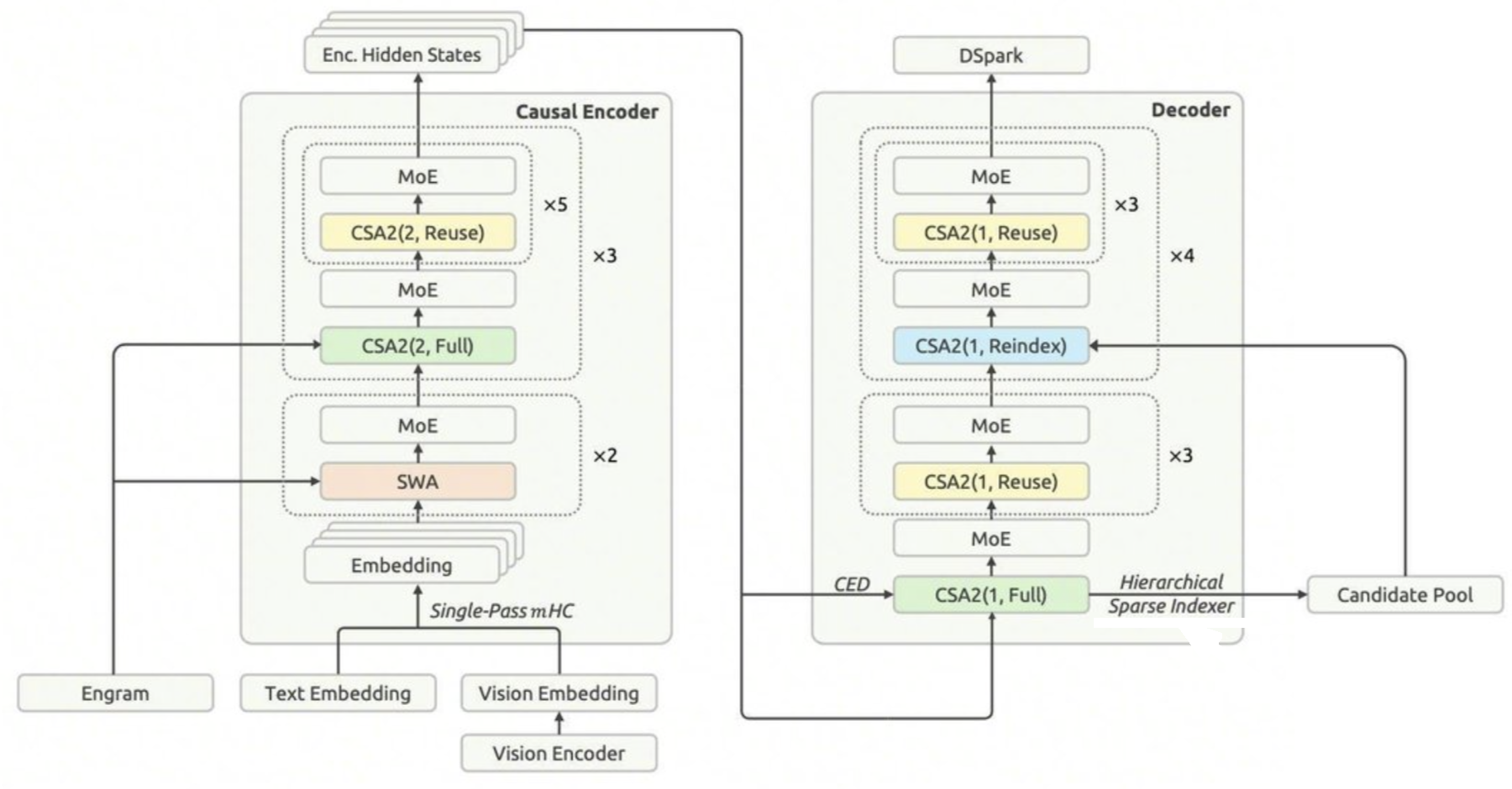
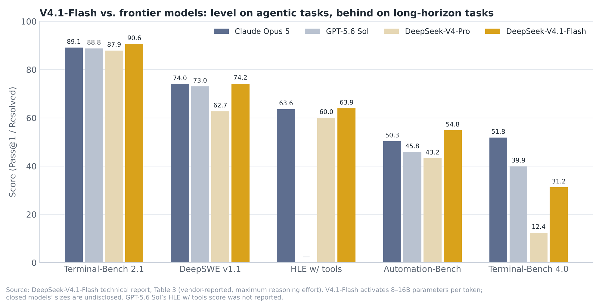
Performance and price: DeepSeek states that V4.1-Flash-Base reaches the level of V4-Pro-Base with 1/3 the total parameters and 1/4 the activated parameters. Peak pricing is $0.30/M for input, $0.006/M for cached input, and $1.20/M for output, with off-peak at half price. On a third-party composite index, however (40 points on Artificial Analysis, against 51 for Claude Opus 5), it still trails by about 10 points in independent evaluation. Vendor-selected benchmarks and independent composite evaluations must be written up separately. This is itself a living lesson in how “averages mislead.”

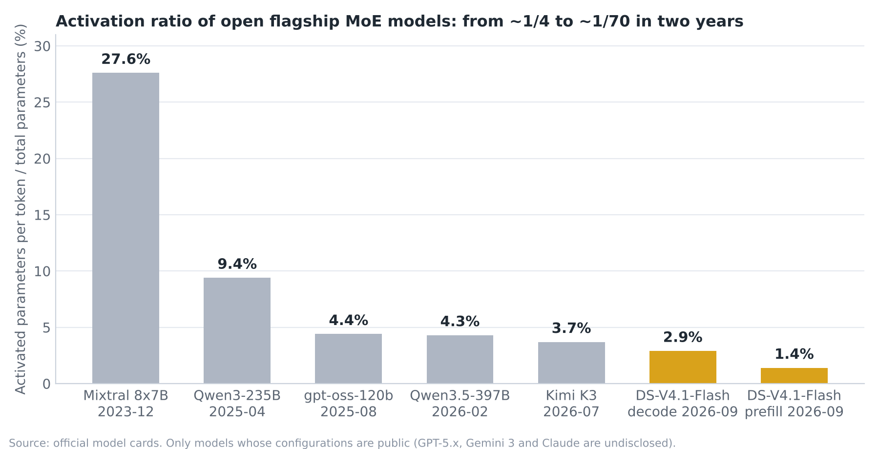
Other major MoE models of 2025–2026 (from official model cards):

Model	Date	Total / activated	Experts (selected / total)	Activation ratio	Other design features
Mixtral 8x7B	2023-12	46.7B / 12.9B	2/8	About 28%	The first high-quality open MoE
gpt-oss-120b	2025-08	116.8B / 5.1B	4/128	4.4%	MXFP4 MoE weights; alternating sliding-window and full attention; attention sink
Qwen3-235B-A22B	2025-04	235B / 22B	8/128	9.4%	—
Qwen3.5-397B-A17B	2026-02	397B / 17B	10+1 / 512	4.3%	Gated DeltaNet linear attention mixed at 3:1, KV reduced to about 1/4
Kimi K2 / K2.5	2025-07 / 2026-01	1.04T / 32B	8+1 / 384	3.1%	MuonClip, no loss spikes over 15.5T tokens
Kimi K3	2026-07	2.8T / 104B	16 / 896, 2 shared	3.7%	KDA linear attention + Gated MLA; MXFP4 QAT
Llama 4 Maverick	2025-04	About 400B / 17B	1 + 1 shared / 128	4.3%	Alternating dense and MoE layers
DeepSeek-V4.1-Flash	2026-09	552B / 8–16B	6+1 / 384	1.4%–2.9%	See above

The trend: in two years the field moved from “2 of 8 experts, 25% activated” to “6–16 experts chosen from several hundred to nearly 1,000, 1.5%–4.5% activated,” with the degree of sparsity rising by roughly an order of magnitude every 1–1.5 years. Shared experts have become standard equipment, and routing now uses auxiliary-loss-free bias, hash routing (the first three layers of V4), and latent-space routing (K3). Among closed models, Google has officially acknowledged that the Gemini 1.5 and Gemini 2.5 series are sparse MoE. GPT-4’s “1.8T MoE” was no more than a 2023 rumor, and the configurations of GPT-5.x and Claude have not been disclosed. At most, write “reportedly.”

Sparsifying attention and the KV cache

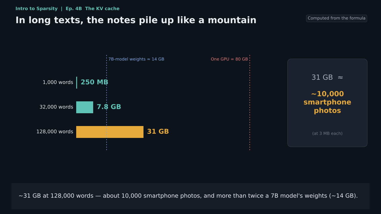
KV cache size = 2 × L × number of layers × number of KV heads × head dimension × bytes per element. Plug in 64 layers, 8 KV heads, a head dimension of 128, FP16, and a 128K context, and the result is about 31 GiB — larger than the weights of many models, and all of it must be re-read every time a single token is generated. There are three countermeasures: reduce the number of KV heads (GQA/MQA), low-rank compression (MLA), and sparse eviction or sparse computation.

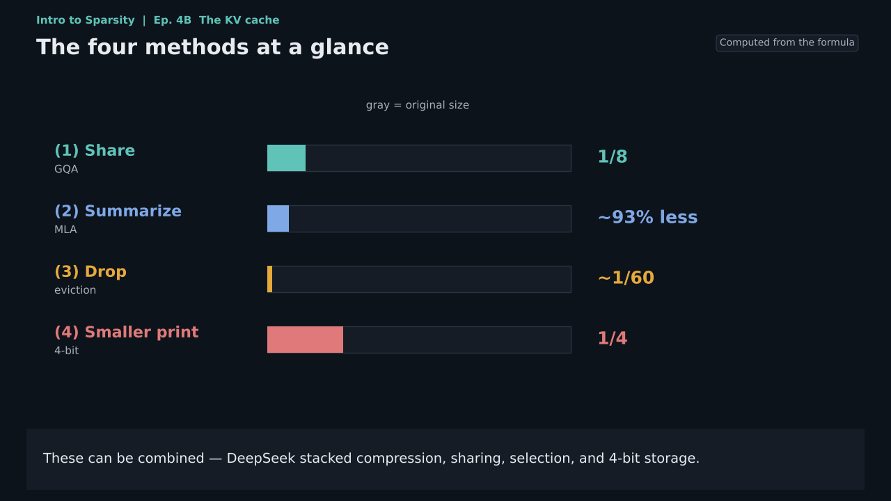
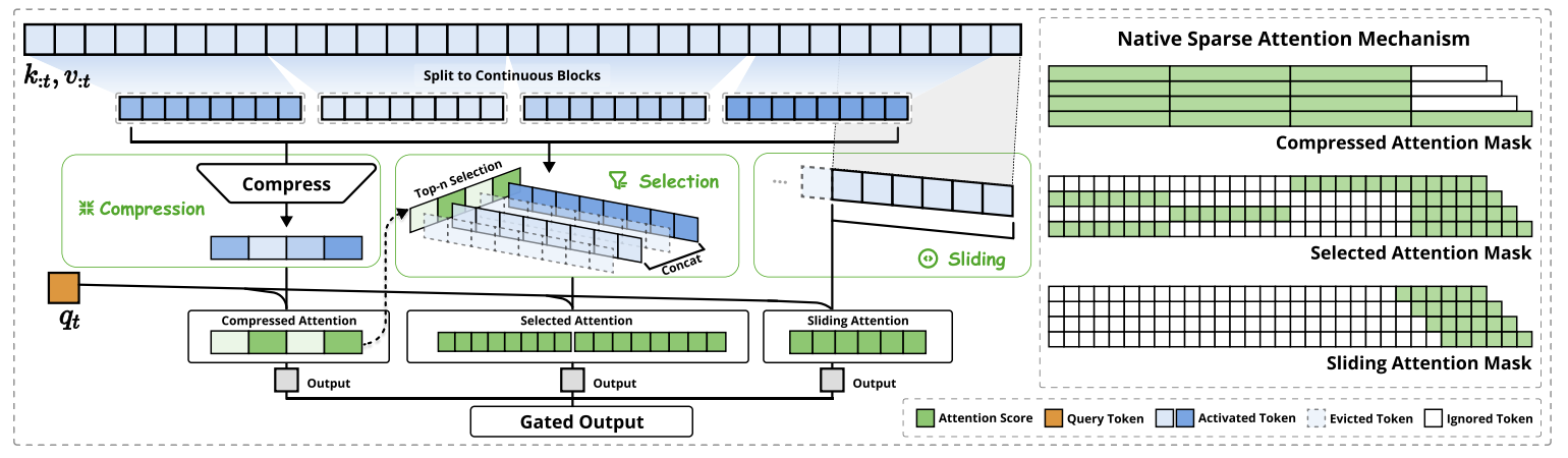
Sparse attention has three generations, and they can be stacked. The first generation uses fixed patterns (Longformer, BigBird, the sliding window in gpt-oss); the second is dynamic eviction at inference time with no retraining required (StreamingLLM, H2O, SnapKV, Quest); the third learns sparsity natively during training (NSA, MoBA, DSA, CSA2). NSA (Yuan et al., DeepSeek × Peking University × the University of Washington) won the Best Paper Award at ACL 2025 and, at a length of 64K, sped up decoding 11.6×, the forward pass 9.0×, and the backward pass 6.0× relative to full attention.

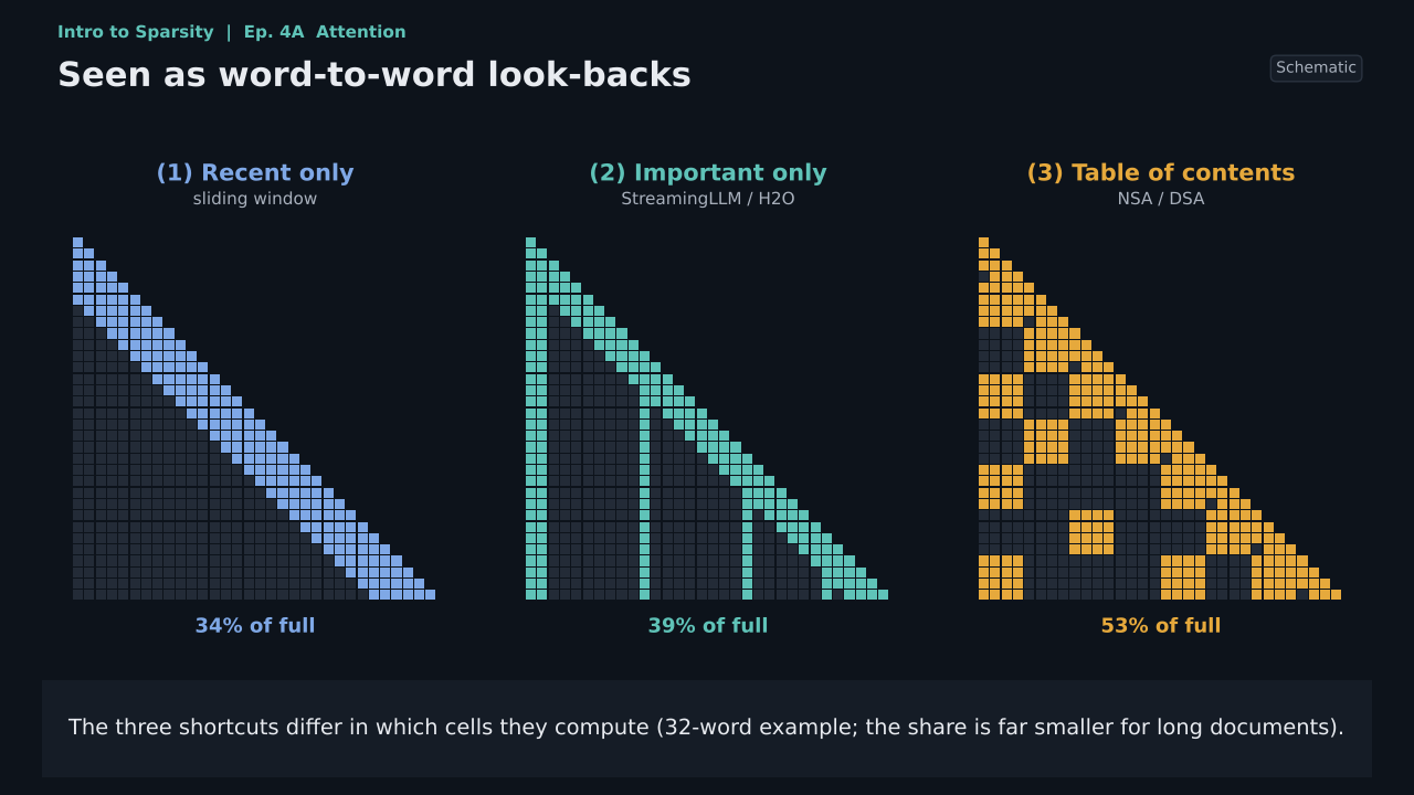
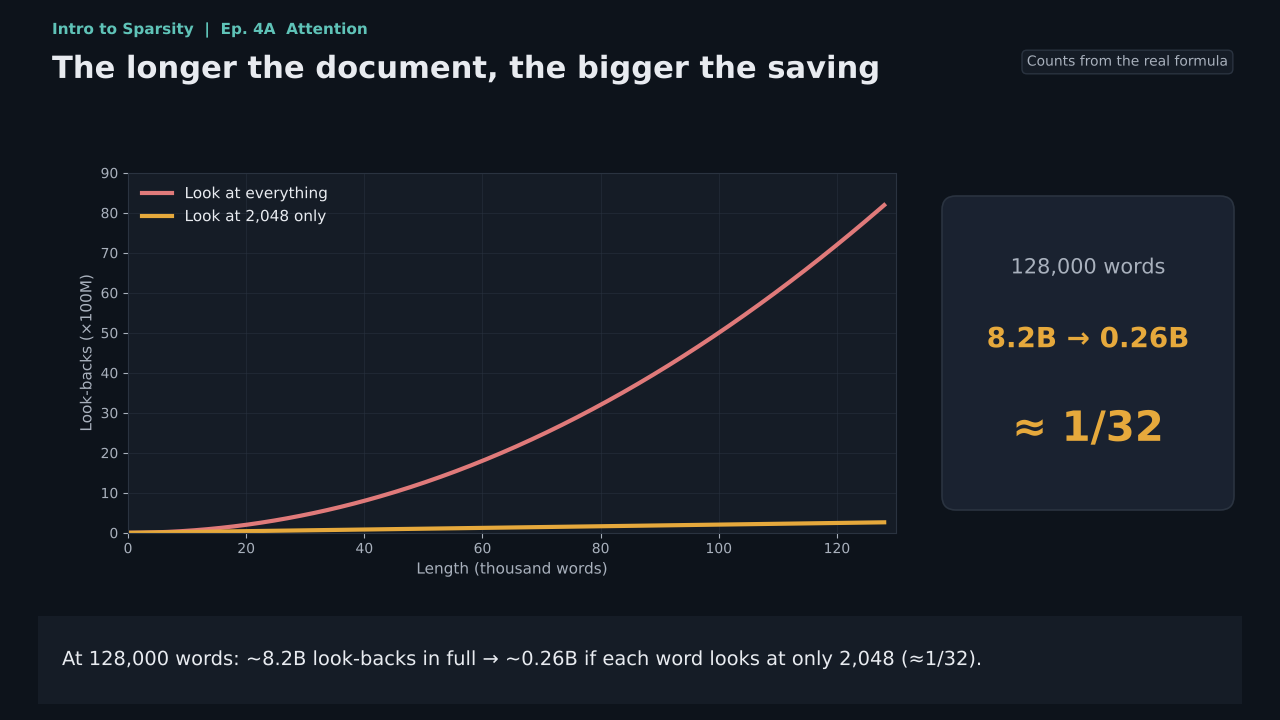
A cold shower from large-scale measurement. Nawrot et al.’s The Sparse Frontier (arXiv:2504.17768, formally published in Findings of ACL 2026) evaluated training-free sparse attention on Qwen2.5 7B–72B, at 16K–128K, across nine tasks, and reached four conclusions. For very long sequences, “large and sparse” beats “small and dense,” and the crossover sits around 32–64K. The optimal sparsity for prefill is 0.80–0.93 (a budget of 1/5–1/15), and decoding is more tolerant. Almost every configuration suffers a large performance drop on at least one task. Sparse attention is no panacea. And no single strategy is best across all tasks and phases. This result is precisely the motivation that gave rise to the third generation’s “natively learnable sparsity.”

Activation sparsity

Q-Sparse (Wang, Ma, Wang & Wei, arXiv:2407.10969) applies top-k directly to the activations of every linear layer, backpropagates with STE, and demonstrated a scaling law for sparsity. The optimal sparsity ratio is about 45.58% for full-precision models and about 61.25% for 1.58-bit models, and at roughly 40% sparsity the model matches a dense model of the same size. When Mistral 7B was further trained on 40B tokens, Q-Sparse scored 63.7 with 3.8B activated parameters, against 64.6 for the dense baseline (7.0B). In ablations, removing STE or replacing top-k with ReLU each caused a clear drop in performance; moreover, with ReLU the sparsity ratio fell as training progressed, whereas with top-k it held constant. This supports the claim that “sparsity should be an architectural constraint, not a regularization term.” TEAL, ReLU Strikes Back, Deja Vu, and PowerInfer form the main lineage on the edge side.

Sparsity in interpretability: the rise of SAEs and the doubts

Anthropic’s path runs as follows. Towards Monosemanticity (2023) used sparse autoencoders to extract monosemantic features from a one-layer model. Scaling Monosemanticity (2024) trained SAEs with up to 34 million features on Claude 3 Sonnet and demonstrated feature clamping with Golden Gate Claude. Circuit Tracing and On the Biology of a Large Language Model (2025) built attribution graphs with cross-layer transcoders and traced multi-step reasoning in Claude 3.5 Haiku. At OpenAI, Gao et al. (2024) trained a 16-million-feature TopK SAE on GPT-4. This lineage is a direct descendant of Olshausen–Field dictionary learning.

The doubts arrived in a cluster in 2024–2025: feature absorption (Chanin et al. 2024); features that are not one-dimensional and linear (Engels et al. 2024); failure to beat a logistic-regression baseline on 113 probing datasets (Kantamneni et al. 2025); and different SAEs finding different features (Leask et al. 2025). In March 2025, Google DeepMind’s mechanistic interpretability team announced that it would “deprioritize fundamental SAE research for now,” saying the field had overinvested in SAEs. The relatively moderate consensus is that SAEs are well suited to discovering unknown concepts but not to serving as detectors or controllers for known ones. New work such as SharedSAE and WriteSAE continues to appear in 2026, but no new unifying consensus has emerged.

A unifying theory: three operators and learning top-k

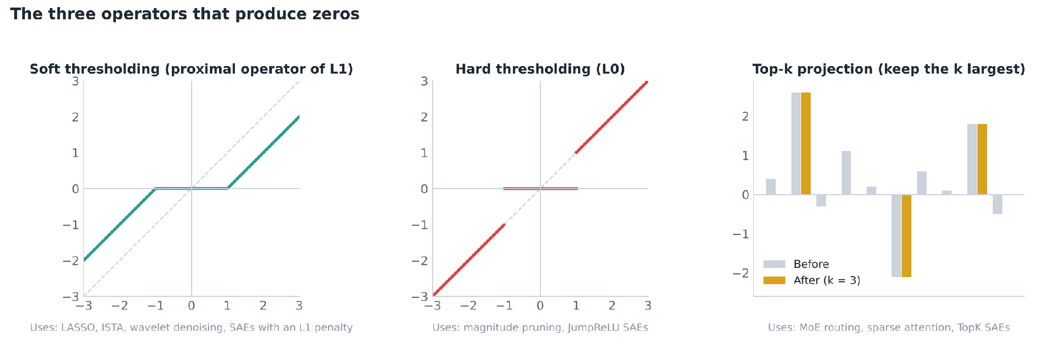
Whether in LASSO, pruning, SAEs, or MoE routing, the step that “produces zeros” is one of three operators.

S_λ(y) = sign(y) · max(|y| − λ, 0), H_τ(y) = y · 1[|y| > τ], P_k(y) = keep only the k largest-magnitude entries

Soft thresholding is the proximal operator of L1 (LASSO, ISTA, wavelet denoising, SAEs with an L1 penalty); hard thresholding corresponds to L0 (magnitude pruning, JumpReLU SAEs); and top-k is the projection onto the set of k-sparse vectors (MoE routing, sparse attention, TopK SAEs, Q-Sparse). ReLU itself is a one-sided hard threshold with τ=0. Nearly all modern large models use the third, because it pins the compute per token to an exact constant, which makes static memory planning and dedicated kernels possible. In the era of large models, sparsity has changed from a “regularization term” into an “architectural constraint.”

Top-k is not differentiable. ∂TopK/∂s is zero almost everywhere, so gradients reach only the gate weights of the selected experts, and the rest can never learn. There are four kinds of engineering fixes. Backpropagate only through the selected experts and add an auxiliary load-balancing loss (the mainstream approach). Add noise with Noisy Top-k to create exploration (Shazeer 2017). Continuous relaxations such as STE, Gumbel-Softmax, and Soft MoE. And, from DeepSeek-V3 onward, the auxiliary-loss-free bias: rank by s+b while weighting by s, and adjust b according to load, outside the gradient. On the sparse-attention side, NSA selects at the block level so that gradients can flow, and DSA first warms up with dense attention, aligning the indexer to the dense attention distribution, before switching to sparse training.

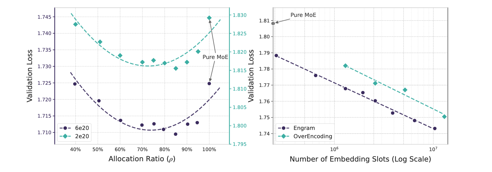
On scaling laws, Clark et al. (2022) unified the scaling of routed models and recommended 64–128 experts. Krajewski et al. (2024) showed that fine-grained experts beat dense models at every compute budget. Frantar et al. (2023) found that the optimal weight sparsity rises with the amount of data. DeepSeek’s Engram paper (arXiv:2601.07372, January 2026) posed the problem of “allocating the sparsity budget” and found a U-shaped law: pure MoE is not optimal, and the best results come when about 20–25% of the sparse parameter budget is allocated to conditional memory. Nine months later, that finding was built into the V4.1 product.

Economics and industry

• The DeepSeek shock. On January 27, 2025, Nvidia closed down about 17%, erasing roughly $589 billion (Bloomberg) to $593 billion (Reuters) in market capitalization — the largest single-day loss of market value in the history of the US stock market.

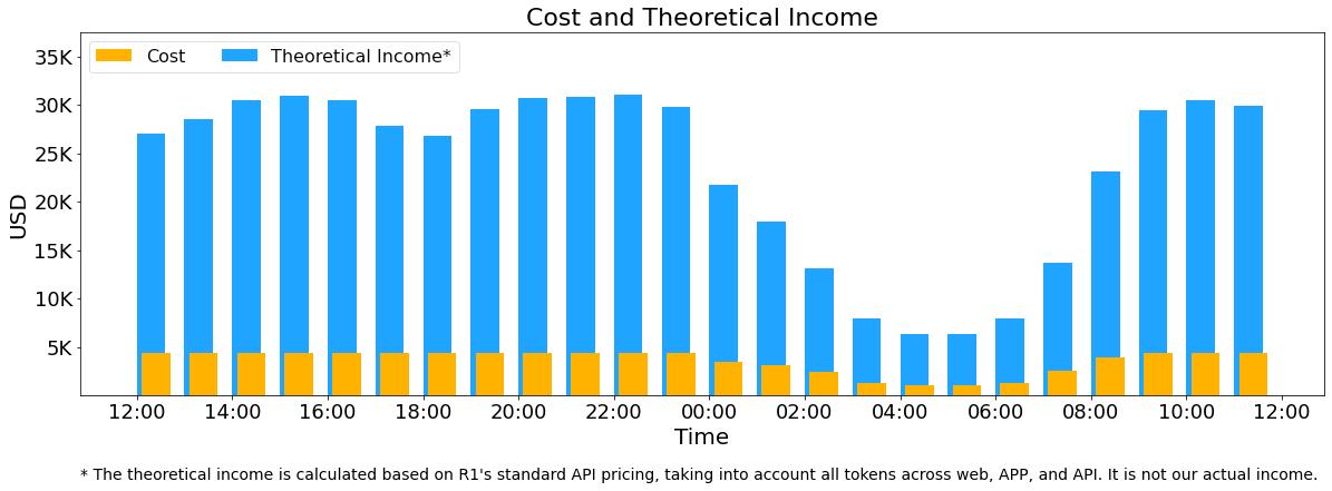
• A 545% theoretical profit margin. On March 1, 2025, DeepSeek disclosed that, pricing an H800 at $2 per hour, its daily cost was $87,072, and that if everything were billed at R1 prices its theoretical daily revenue would be $562,027. It stated explicitly that actual revenue is far lower and that R&D and training costs are not included. Always attach the word “theoretical” when citing this figure.

• Inference prices. Epoch AI (March 2025) noted that the price of inference at a fixed level of capability is falling by 9× to 900× per year, with the rate varying by task. Yet enterprises’ total bills keep rising, because agents multiply the number of calls per task many times over.

• The economics of MoE inference. Memory is determined by total parameters, and only with large batches and expert parallelism does each expert receive enough tokens. MoE is inherently suited to large centralized services, not to small-scale self-hosting. vLLM and SGLang supported MLA, DSA, and V4.1 from the day each was released.

A systematic comparison of each lab’s approach

Lining up the labs on the same criteria shows that there is no single path to sparsification; several strategies are competing in parallel.

Lab	Disclosure of configuration	Main kind of sparsity	Experts (selected / total)	Attention strategy	KV strategy	Weight format	Representative models	Distinguishing features
DeepSeek	Public, with technical reports	MoE + sparse attention + conditional memory	6/384 + 1 shared	Native sparse (DSA → CSA2), trained from the start	MLA low-rank + FP4 + cross-layer reuse, 890 B/token	FP4/FP8 experts	V3, V3.2, V4, V4.1-Flash	Stacks three axes of sparsity; encoder–decoder division of labor for agents
Moonshot (Kimi)	Weights and reports public	MoE + linear-attention hybrid	16/896 + 2 shared	Block-sparse MoBA; K3 uses KDA linear attention + Gated MLA	No KV for the linear layers	MXFP4 QAT	K2, K2.5, K3	Largest expert count; stable training with MuonClip
Alibaba (Qwen)	Model cards public	MoE + linear-attention hybrid	10/512 + 1 shared	Gated DeltaNet and Gated Attention at 3:1	KV cut to about 1/4	BF16/FP8	Qwen3, Qwen3.5	Full series from edge to flagship
Meta	Model cards public	MoE	1/128 + 1 shared (Maverick)	Alternating dense and MoE layers; iRoPE	Standard GQA	BF16	Llama 4	10M context (Scout); Behemoth unreleased
OpenAI	Only gpt-oss public	MoE	4/128	Alternating sliding window (128) and global attention; attention sink	GQA, 8 heads	MXFP4	gpt-oss-120b/20b	GPT-5.x undisclosed; SAE research (Gao 2024)
Google	Gemini 1.5 and 2.5 officially confirmed as MoE; details undisclosed	MoE; elastic structure for the edge	Undisclosed	Undisclosed	Undisclosed	Undisclosed	Gemini 1.5/2.5, Gemma 3n	MatFormer nested submodels, PLE
Anthropic	Undisclosed	Sparsity for interpretability (SAEs, transcoders)	Undisclosed	Undisclosed	Undisclosed	Undisclosed	Claude series	Uses sparsity as a tool for “understanding the model”
Mistral	Weights public	MoE	2/8	Standard	GQA	BF16	Mixtral 8x7B/8x22B	First high-quality open MoE (December 2023)
Microsoft Research	Papers public	Activation sparsity + 1.58-bit	—	Standard	Standard	1.58-bit (BitNet)	Q-Sparse, BitNet b1.58	Combines sparsity with extreme low-bit quantization
Meituan / Ant / Zhipu	Model cards public	MoE variants	Various	Various	Various	Various	LongCat-Flash, Ling, GLM-4.5/4.6	Zero-compute experts, shortcut-connected MoE

Three observations follow. First, the main source of innovation in sparse architectures is the Chinese open-model camp. Fine-grained experts, shared experts, auxiliary-loss-free load balancing, native sparse attention, conditional memory, and linear-attention hybrids were almost all first published by DeepSeek, Qwen, and Kimi. Second, the configurations of the big closed labs are black boxes, and can only be inferred from public information such as the gpt-oss and Gemini reports. Citing “GPT-4 is a 1.8T MoE” as fact is a common error. Third, attention is splitting into two paths. DeepSeek chose “sparse attention” (computing only some pairs of tokens); Qwen and Kimi chose “linear-attention hybrids” (replacing the KV cache with a recurrent state). Both attack the same problem — the memory and bandwidth of the KV cache — but with different mathematical tools: the former is sparse, the latter closer to low-rank recurrence.

The systems stack: the engineering that makes sparsity actually run

Whether the gains of a sparse architecture are actually realized is decided in a layer that is easy to overlook: systems software.

• Expert parallelism and communication. DeepEP (released by DeepSeek in 2025) provides high-throughput, low-latency all-to-all kernels that support FP8 and RDMA over NVSHMEM, and overlaps communication with computation. MegaBlocks (2023) rewrote MoE computation as block-sparse GEMM to achieve dropless MoE, 2.4× faster than dense Megatron-LM.

• Attention kernels. FlashMLA is optimized for MLA. DSA and CSA2 require matching indexer and sparse-attention kernels, which DeepSeek released in FlashMLA and DeepGEMM. The three modes of CSA2 in V4.1 mean the inference engine must manage cross-layer reuse of KV and indexes.

• Inference frameworks. vLLM and SGLang supported MLA, DSA, and V4.1-Flash from the day of release, covering H100/H200/B200/GB200 and AMD MI355X. NVIDIA NeMo AutoModel provides a fine-tuning recipe for V4.1, which requires 64 GPUs in a single NVLink domain.

• Tiered storage. V4.1’s Engram table (about 183 GiB) is designed to sit in host memory and be prefetched over RDMA. Papers already exist that hold Engram in a CXL memory pool, moving “knowledge” from HBM to a cheaper tier. SWA Bounded Replay avoids persisting sliding-window KV to SSD.

• Quantization formats. MXFP4 (one shared 8-bit scale per 32 elements, 4.25 bits on average) became the de facto standard for MoE expert weights in 2025–2026. Blackwell natively supports FP4 tensor cores.

The conclusion of this section echoes “The Neural Network Era.” Every victory for sparsity has come with kernels and scheduling to match. 2:4 sparsity never spread because, tensor cores notwithstanding, it lacked a mature end-to-end software stack. MoE became mainstream because it had DeepEP, MegaBlocks, and vLLM.

Where Sparsity Meets Deep Learning: Recent Advances in Imaging and Signal Processing

While large models used sparsity to save computation, imaging and signal processing took a different road: combining sparse priors with deep networks to recover signals from incomplete, noisy measurements. The results flowed back the other way, shaping how large models are interpreted and how their architectures are designed.

Algorithm unrolling: turning iterative sparse solvers into networks

The starting point is LISTA, by Gregor and LeCun (2010). It “unrolls” the fixed iterations of ISTA into a network with a finite number of layers whose parameters can be learned. Each layer is still “a linear transform plus soft thresholding,” but the matrices and thresholds are learned from data. The result converges one to two orders of magnitude faster than hand-tuned ISTA, and it keeps an interpretable structure: each layer corresponds to one step of a proximal gradient method. Algorithm unrolling went on to become the mainstream framework in computational imaging. ADMM-Net and ISTA-Net are used to reconstruct compressed-sensing MRI, and unrolled networks have outperformed classical CS methods on clinically undersampled data. The deeper significance of unrolling is that it showed deep networks can be read as learnable versions of sparse solvers, an insight that later supplied the intuition for decoding neural networks with sparse dictionaries.

Plug-and-play priors and regularization by denoising

Classical regularization (L1, total variation) writes the prior down as an explicit penalty term. The plug-and-play (PnP) framework that emerged from 2013 onward discovered that the “apply the proximal operator” step in ADMM or proximal gradient methods can be replaced by an arbitrary denoiser, which is to say a trained deep denoising network. The prior went from “a single formula” to “a black-box denoiser,” and the sparsity prior became just one special case. Regularization by Denoising (RED) and, later, diffusion-model priors carry on this lineage. In this view, soft-thresholding denoising, BM3D, and deep denoisers are three generations of interchangeable parts that slot into the same position.

Deep Image Prior: the network’s structure is itself the prior

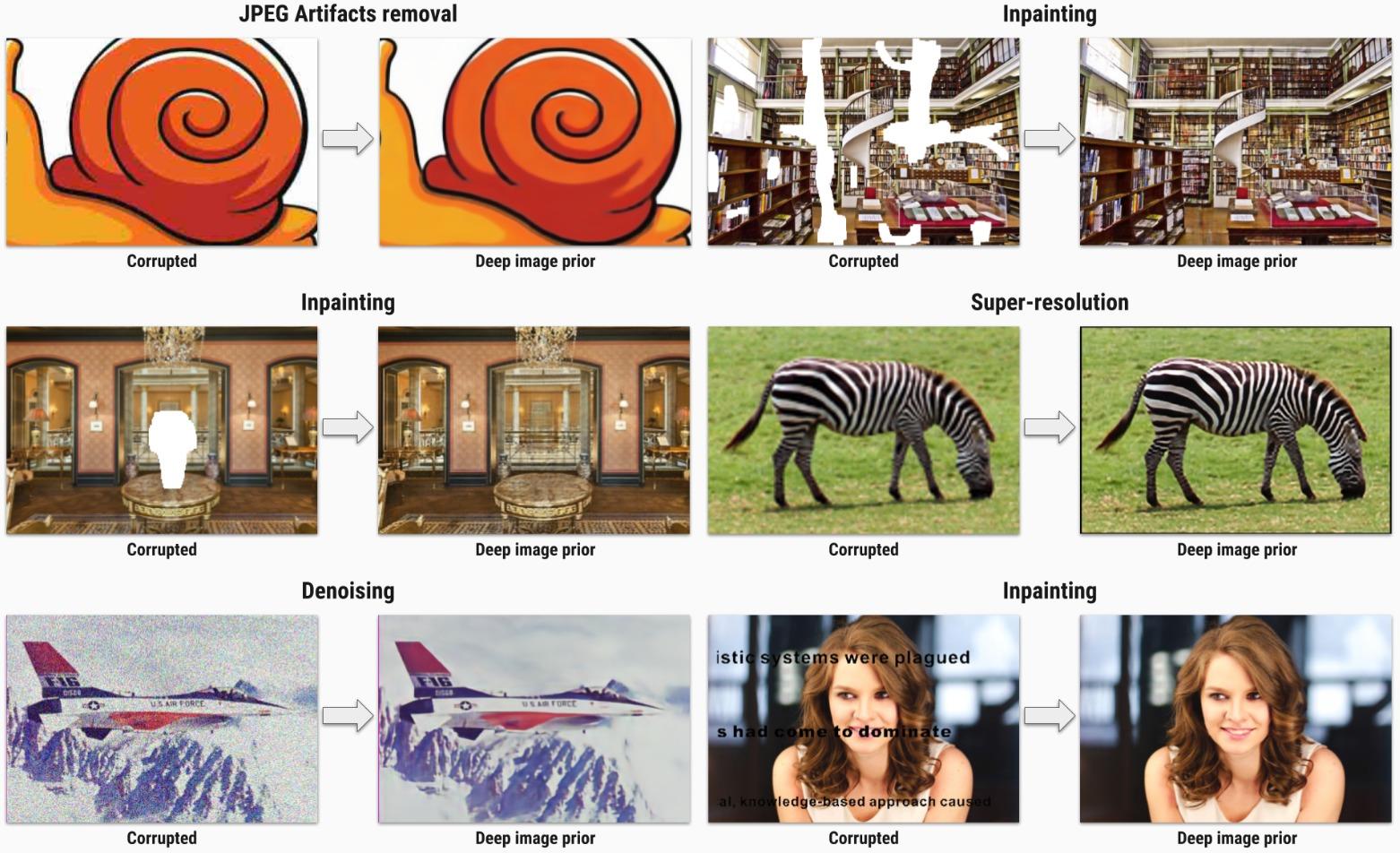
The Deep Image Prior of Ulyanov, Vedaldi, and Lempitsky (2018) delivered a counterintuitive result. Fit a randomly initialized, untrained convolutional network to a single degraded image, and it can denoise, super-resolve, and inpaint. The structure of a convolutional network favors the low-frequency, self-similar statistics of natural images, and it fits noise only slowly, so stopping early yields a clean image. This connects directly to the natural image statistics discussed in “Prehistory.” The network’s structure implicitly encodes the prior that natural images are sparse in some basis; the only difference is that the basis is no longer written out explicitly. Since DIP, “structure is the prior” has become a key lens for understanding the inductive biases of neural networks, and a bridge to classical sparse theory. DIP can be seen as a method that does the same thing adaptively with an implicit, learnable “frame”: it keeps only the components that genuinely represent the structure of the signal.

Learned dictionaries and structured frames

Between fixed wavelets, the unstructured dictionaries learned by K-SVD, and the implicit priors learned by deep networks, there is a middle road: preserve the mathematical structure of tight frames and unitary transforms (perfect reconstruction, energy preservation) while learning their parameters from data. Non-separable oriented symmetric lapped transforms (NSOLT) and lattice-structure unitary networks (LSUN) belong to this category. By constraining the transform to the manifold of tight frames and parameterizing it with a lattice structure, they keep the interpretability and invertibility of classical transforms while gaining adaptability to specific data. The value of this road is being rediscovered in the era of large models. SAEs need overcomplete dictionaries, and MLA needs invertible low-rank projections. Both are searching for a balance between structural constraints and adaptation to data, the very design problem that structured frames have confronted all along.

Three points of contact with large models

First, SAEs are sparse coding itself. Anthropic’s sparse autoencoders are mathematically identical to Olshausen–Field dictionary learning; only the data has changed, from image patches to residual-stream activations. Second, algorithm unrolling anticipated the reading “network = solver.” Anthropic’s transcoders and attribution graphs are, in essence, a search for a sparse, legible alternative computational graph for the Transformer. Third, the idea of structural priors has entered architecture design. MoE expert blocks, the cross-layer reuse in CSA2, and Engram’s lookup tables all write the belief “the data must have this structure” into the shape of the network itself rather than into the loss function. This is the imaging-world counterpart to the conclusion of the section “A unifying theory”: sparsity has shifted from a regularization term to an architectural constraint.

Applications: Where Sparsity Has Truly Created Value

Sparsity creates value where there is a great deal to process but only a little that truly matters. Reviewing long documents is one of the most typical examples.

• LLM inference in the cloud. Nearly all of the low-priced frontier APIs of 2026 come from highly sparse MoE models. DeepSeek-V4.1-Flash’s off-peak output costs $0.60/M, and gpt-oss-120b runs about $0.03/M for input and about $0.17/M for output on OpenRouter.

• Long context and agents. In the V4.1 announcement, DeepSeek stated plainly that cache-hit charges often account for the bulk of an agent’s cost, and that compressing the cache can cut this part substantially. The price of cached input ($0.006/M) is 1/50 of the cache-miss price ($0.30/M), and this is the central lever in the economics of agents.

• Edge. Apple’s LLM in a Flash (2023) loads sparsely activated parameters from flash storage on demand. Gemma 3n uses MatFormer’s nested submodels and per-layer embeddings (PLE). MoE models with 3B activated parameters, such as Qwen3.5-35B-A3B, have become candidates for the browser and the edge.

• Multimodal. V4.1 gives image tokens a dedicated routing bias. Visual tokens are numerous and highly redundant, which makes them an ideal target for sparse attention.

• Science and medicine. CS-MRI has shortened average scan times in routine clinical practice by about 20%, and by 23%–43% for a single sequence. The SMILI pipeline behind the EHT’s black-hole imaging is built on sparse modeling.

Enterprise review of long documents and drawings (directly relevant to our business)

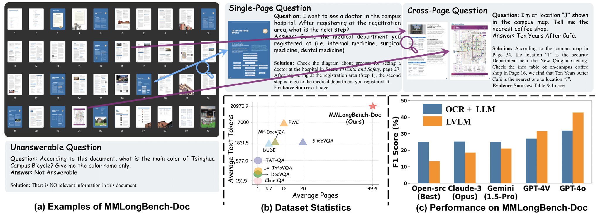
The benchmark for difficulty. MMLongBench-Doc (NeurIPS 2024 D&B) collects 135 PDFs averaging 47.5 pages and roughly 21,000 tokens of text, with 1,082 expert-written questions. Of these, 33.2% require cross-page evidence, and 22.8% are designed to be unanswerable in order to detect hallucination. Human annotators score an F1 of 66.0%, and 12 of the 14 vision-language models perform worse than when OCR text is fed to the corresponding text-only model. LongDocURL’s 396 documents average 86 pages, and 52.9% of its questions are cross-page. The length of these documents and their share of questions that span pages and elements closely resemble building-permit applications (drawings, structural calculations, and application forms running from several dozen to well over 100 pages).

The bottleneck is not context length alone. It is choosing the right top-K among scattered evidence. Retrieval (selecting the top-K pages) and sparse attention (selecting the top-K token blocks) are mathematically the same operator; the difference is whether the selection happens outside the model (auditable, able to cite provisions) or inside it (end-to-end and opaque).

Limits. Sparse Frontier shows that sparse attention can degrade performance on individual tasks even at moderate sparsity. In review work, “clause X contradicts the dimension noted on page 37” is exactly the kind of task where you “miss one and the whole answer is wrong.” A hybrid of retrieval plus re-verification in a long context is therefore safer than betting on either one alone. The 2025 research on multi-page documents, including SimpleDoc, MDocAgent, and LAD-RAG, takes this road as well.

Benefits and Costs

For weight sparsity, “sparsity is overrated” is broadly true in the LLM era. For conditional computation and attention sparsity, the opposite holds: both are already the default at the frontier. Keeping these two apart is the key to understanding the whole debate.

Benefits

• Cost: activation ratios have fallen to 1.5%–4.5%, and the price curve is dropping fast.

• Decoupling capacity from compute: total parameters set knowledge capacity, activated parameters set the cost per token, and the two can be scaled independently. Engram goes further, moving static knowledge into cheap host memory.

• Long context becomes practical: V4.1’s decode FLOPs rise by only about a quarter between 4K and 1M.

• A tool for interpretability: SAEs and transcoders are used to discover unknown concepts.

Costs and risks

• Memory is set by total parameters: V4.1’s routed experts (MXFP4) take about 259.5 GiB and the Engram table about 183 GiB; sparsity saves no storage.

• Communication overhead: the all-to-all of expert parallelism is the main bottleneck in MoE training, and Engram needs prefetching over RDMA or CXL.

• Training instability and load imbalance: a whole series of patches becomes necessary, among them z-loss, bias adjustment, and hash routing.

• Fine-tuning is hard: routing collapses easily on small datasets. V4.1’s official fine-tuning procedure requires 64 GPUs in a single NVLink domain.

• Evaluation pitfalls: Sparse Frontier’s finding that “almost every configuration loses performance on at least one task.” V4.1 matches the frontier on the vendor’s benchmarks but trails by about 10 points on an independent composite index.

• The limits of SAEs: see the section “Sparsity in interpretability.”

• Weight sparsity still loses on efficiency: conventional methods struggle to break through the 50%–60% sparsity wall.

Representative views (quoted from the sources)

Position	Source	View
Supportive: hardware decides who wins	Hooker 2021	Ideas win “because they are a good fit for the software and hardware available, not because the idea is superior”
Supportive: a new axis of sparsity	DeepSeek, Engram 2026	“We believe conditional memory will become an indispensable modeling primitive for the next generation of sparse models”
Cautious	Nawrot et al. 2026	“Sparse attention is not a silver bullet”
Negative	Google DeepMind 2025	“We don’t expect SAEs to be a game-changer for interpretability, and we suspect the field has over-invested in them”
Middle ground	arXiv:2506.23845	SAEs are poor at acting on known concepts, but they are a powerful tool for discovering unknown ones

A verdict on each of the five kinds of sparsity (September 2026)

There is no single answer to “is sparsity overrated?”; the question has to be answered kind by kind.

Kind of sparsity	Status in 2026	Verdict	Main evidence
Weight sparsity (unstructured pruning)	Active research, very little industrial deployment	Overrated in the LLM era; quantization won	The 50%–60% sparsity wall; no efficient GPU kernels; MXFP4 is the de facto standard
Structured sparsity (2:4, block)	Hardware support exists, but end-to-end speedups are limited	Partly realized; block sparsity won in the form of MoE	2:4 rarely approaches 2× in measured results; MegaBlocks’ block-sparse GEMM became the foundation of MoE
Activation sparsity (ReLU, top-k activation)	Attention at the edge and in research; absorbed into MoE in the cloud	Potential underrated, but the main battleground is the edge	Q-Sparse matches dense at about 40% sparsity; TEAL and PowerInfer target memory-constrained devices
Conditional computation (MoE)	The default architecture at the frontier	Lives up to its reputation, and still deepening	Activation ratio fell from 25% to 1.5%–4.5% in two years; adopted by every flagship-class open model of 2025–2026
Attention sparsity	Natively trainable versions are in products	Established, but with a risk of per-task performance drops	NSA won the ACL Best Paper Award; V4.1 trains it from the start; Sparse Frontier’s “drop on at least one task”
(Parallel line) Low rank	MLA and LoRA are widely used	Established, but should not be confused with sparsity	Low-rank KV compression of up to about 93% (V2); LoRA is the standard for fine-tuning
(Tool) Sparse dictionaries / SAEs	Under debate	Established as a discovery tool; overrated as a detector or controller	GDM deprioritized it; trails linear probes on 113 datasets; Anthropic moved to transcoders and attribution graphs

In one sentence: sparsity won on “activation” and “attention” and lost on “weights.” It won not because the theory was superior, but because the positions of the zeros had a structure the hardware could exploit.

The Future (2026–2030)

The next axis of sparsity is no longer “which parameters to compute” but “which knowledge to store, and which history to read.” Below are the research frontier, the hardware trends, and five falsifiable predictions.

The research frontier

• Multi-axis sparsity and budget allocation. The U-shaped law found in the Engram paper shows that pure MoE is not optimal and that the sparsity budget should be split between “experts” and “conditional memory.” The 27B Engram model achieved MMLU +3.4, BBH +5.0, and HumanEval +3.0 over an MoE baseline with the same parameter count and the same FLOPs. Mechanistic analysis shows that conditional memory frees the early layers from having to reassemble static knowledge.

• Natively trainable sparsity becomes the default. V4.1 trains sparse attention from scratch at 64K, with no dense warm-up beforehand. It shows that sparse attention has gone from an inference-time approximation to a first-class citizen at training time.

• Sparsity × inference-time compute. Reasoning models produce long outputs, and both prefill and decode are heavy. MoE provides knowledge capacity; long chains of thought provide reasoning depth. CED’s asymmetric activation is a trade-off aimed at workloads with different read/write ratios.

• Modularity and continual learning. Experts and memory tables can be edited locally. For example, there is research that writes a user’s memory as a local parameter edit (User as Engram, arXiv:2606.19172).

• Combining sparsity with quantization. MXFP4 experts, FP4 KV, and FP8 Engram are already used together in V4.1 and K3. Q-Sparse’s conclusion is that the more aggressive the quantization, the higher the optimal degree of sparsity.

• Co-design with hardware. Blackwell supports FP4 natively, and tiered KV storage using CXL memory pools and SSDs is advancing. Neuromorphic computing at LLM scale remains a distant prospect.

Five falsifiable predictions (with rationale)

Prediction	Deadline	Rationale
Global KV falls to 500 bytes per token or less in at least one major open model	End of 2027	A 437× reduction from V1 to V4.1, a 4× reduction in the single generation from V4 to V4.1, and FP4 already in use
At least three of the top five open models have an activation ratio per token below 3%	End of 2027	In 2026 there are already V4.1 (2.9%), K3 (3.7%), and Qwen3.5 (4.3%), and expert counts double every generation
At least two major labs other than DeepSeek introduce lookup-table-style conditional memory into their flagship open models	2028	Engram already has CXL, SSD, and training-free derivative work, and it has landed in NeMo
SAEs do not become an officially announced primary production safety-monitoring method at any frontier research lab	2028	GDM’s deprioritization; negative results on downstream tasks
The API unit price for a fixed level of capability keeps falling by 10× or more per year, but enterprises’ agent spend per task rises	Ongoing	Epoch’s price trends; the doubling of agent call counts

What This Means for Us

Review is, in essence, the task of selecting the top-K out of a vast number of provisions and pages, and what the sparsification trend is driving down is precisely the unit cost of this kind of task. For a company building a review agent for long documents and drawings, there are four actionable implications.

• The cost curve. Treat “cache hit rate” and “share of off-peak batch processing” as first-class metrics. Review tasks are inherently batchable and can run offline. Place stable laws and ordinances at the front of the prompt to maximize prefix-cache hits. V4.1’s cached-input price is 1/50 of the cache-miss price, and off-peak halves it again.

• Model selection. Choose models on our own evaluation set for “cross-page matching and clause citation,” and judge by the score on the hardest subtask, not the average. Use a highly sparse open MoE as the main workhorse model, and a closed frontier model to double-check the difficult cases.

• Long-context strategy. Adopt a hybrid: “retrieval of the top-K pages (auditable, with citations) + re-checking in a 1M context (to avoid missing cross-page relationships).” Sparse Frontier’s conclusion applies here directly. Betting on sparse attention alone drops performance on some tasks, and review is exactly a “miss one and the whole answer is wrong” task.

• The self-hosting decision. MoE memory is set by total parameters; V4.1’s routed experts plus the Engram table exceed 440 GiB, and the official fine-tuning procedure requires 64 GPUs in a single NVLink domain. At a scale of fewer than a few dozen GPUs it almost never pays off, so prefer the API.

A research opportunity. Existing work treats “which pages to check within a budget” as a retrieval problem. But the truly sparse object in cross-page consistency checking is not the “page” but the “page pair.” P pages have P(P−1)/2 pairs, and from these we select k pairs to cross-check. This maps directly onto the sparse coordination graphs of multi-agent systems, and it is isomorphic to the idea behind DSA, which scores every (query, key) pair with a lightweight indexer and takes the top-k. It is a direction where we can differentiate and cut in.

Appendices

A. Timeline (1948–September 2026)

Year	Event	Reliability
1948	Shannon, A Mathematical Theory of Communication: redundancy and entropy formalized	primary paper
1961	Barlow’s redundancy reduction hypothesis	primary paper
1967	Tinney & Walker’s sparse-matrix ordering (power-grid computation)	primary paper
1978	Rissanen’s minimum description length (MDL)	primary paper
1987	Field: natural image statistics and cortical receptive fields	primary paper
1988–89	Daubechies’s compactly supported orthogonal wavelets; Mallat’s multiresolution analysis	primary paper
1990–93	Pruning via OBD / OBS; Matching Pursuit	primary paper
1991	Jacobs–Jordan–Nowlan–Hinton’s mixtures of local experts	primary paper
1992 / 2000	JPEG / JPEG2000	standard
1994–96	Wavelet thresholding denoising; Breiman’s garrote; LASSO; Olshausen & Field’s sparse coding	primary paper
1998	Basis Pursuit; DeVore’s nonlinear approximation	primary paper
2001–03	Attwell & Laughlin’s energy budget; Lennie’s “possibly fewer than 1%”	primary paper (verified)
2004–05	LARS; Elastic Net	primary paper
2006–07	Compressed sensing; K-SVD; Lustig’s CS-MRI	primary paper
2009	Donoho–Tanner phase transition	primary paper
2011	Glorot’s ReLU (50–85% exact zeros); Robust PCA	primary paper (verified)
2012	Google’s cat-face neuron	primary paper (verified)
2013–14	Bengio’s conditional computation and the STE; Gavish–Donoho optimal hard threshold	primary paper
2016	Deep Compression	primary paper
2017	Shazeer’s sparsely-gated MoE (a 137B MoE layer)	primary paper (verified)
2019	The lottery ticket hypothesis; EHT M87*; Sartoretti’s clinical study of CS-MRI	primary paper
2020	GShard; Hooker’s Hardware Lottery; Ampere’s 2:4	primary paper
2021–22	Switch Transformer; GLaM; ST-MoE; Expert Choice; Clark’s MoE scaling	primary paper
2023	Mixtral; SparseGPT / Wanda; StreamingLLM / H2O; Towards Monosemanticity	primary paper
Jan–Feb 2024	DeepSeekMoE; Gemini 1.5 officially confirmed as MoE	technical report
May 2024	DeepSeek-V2 (MLA); Scaling Monosemanticity; Golden Gate Claude	technical report
Jun–Jul 2024	Gao’s TopK SAE; Q-Sparse	primary paper (verified)
Dec 2024	DeepSeek-V3 (671B/37B)	technical report
Jan 27, 2025	The DeepSeek shock: Nvidia’s market capitalization falls by roughly $589 billion in a single day	reliable press reports
Feb–Mar 2025	NSA, MoBA; a theoretical profit margin of 545% for the inference system; GDM lowers the priority of SAEs	primary paper / official
Apr 2025	Qwen3 MoE; the Sparse Frontier preprint; Llama 4	official / primary paper
Jul–Aug 2025	NSA wins the ACL Best Paper Award; Kimi K2; gpt-oss	official
Sep–Dec 2025	DeepSeek-V3.2, DSA	technical report
Jan 2026	Engram: conditional memory and a U-shaped sparsity budget allocation	primary paper
Feb 2026	Qwen3.5-397B-A17B	official model card
Apr 24, 2026	DeepSeek-V4 (Pro 1.6T/49B, Flash 284B/13B)	technical report
Jul 2026	Kimi K3 (2.8T/104B); Sparse Frontier published in Findings of ACL 2026	official
Sep 10, 2026	DeepSeek-V4.1-Flash (CED, CSA2, 890 B/token, Engram)	official + technical report (verified)

B. Data series that can be charted

• DeepSeek’s global KV cache (per token): V1 ≈ 389 KB (estimated) → V3.2 ≈ 48 KB → V4-Flash ≈ 3.5 KB → V4.1-Flash 890 B. Log scale.

• Activation ratio per token: Mixtral 28% → Qwen3 9.4% → gpt-oss 4.4% → Qwen3.5 4.3% → Kimi K3 3.7% → V4.1 decode 2.9% / prefill 1.4%.

• Number of experts (selected / total): 2/8 → 4/128 → 8/256 → 6/384 → 10/512 → 16/896.

• DeepSeek API prices ($/M, input / output): V4-Flash 0.14 / 0.28; V4-Pro 1.74 / 3.48 (peak-hour output 3.96 from August onward); V4.1-Flash peak 0.30 / 1.20, off-peak 0.15 / 0.60, cache 0.006.

• Sparse Frontier: optimal sparsity for prefill 0.80–0.93; decoding remains practical even at 0.95; the crossover point is 32–64K.

• Sparsity rates in Glorot 2011: MNIST 83.4%, CIFAR10 72.0%, NISTP 68.0%, NORB 73.8%.

• Q-Sparse: optimal sparsity rate 45.58% (full precision) / 61.25% (1.58-bit); on par with dense at around 40%.

• Engram-27B’s gap over the MoE baseline: MMLU +3.4, CMMLU +4.0, BBH +5.0, ARC-C +3.7, HumanEval +3.0, MATH +2.4.

• CS-MRI: scan time −20.2%, examination duration −16%, single sequences −23% to −43%, number of examinations +27%.

• GPU compute and bandwidth: see the GPU table in “The Neural Network Era.”

C. Anecdotes and story material

• How “Lennie’s 1%” became “1–4%”: usable as an opening that corrects a misconception.

• The cat-face neuron (2012): 1,000 machines, over three days, taught themselves “cat” from YouTube frames.

• Outrageously (2017): a 137B MoE layer in the LSTM era foreshadowed the landscape of 2026. The co-authorship of Hinton and Dean is emblematic of “an old idea from 1991 × Google’s compute.”

• The DeepSeek shock (January 27, 2025) and the word “theoretical” attached to 545%.

• Golden Gate Claude (2024) and GDM’s hard brake (March 2025).

• CS-MRI: patients spent 20% less time lying on the scanner table, and hospitals could perform 27% more examinations.

• 437×: the “memory” per token shrank from roughly 389 KB to 890 bytes.

• The return of N-grams: a statistical language model once consigned to history came back to the frontier as Engram.

D. Common misconceptions and their corrections

Common phrasing	Accurate statement
The brain uses only 1–4% of its neurons	Lennie 2003 actually says “possibly fewer than 1%,” an upper-bound estimate based on energy. The 1–4% figure is a secondary citation via Glorot 2011
ReLU networks are 90% sparse	Glorot 2011: about 50% at initialization, 50%–85% after training
GPT-4 is a 1.8T MoE with 16 experts	A 2023 rumor that OpenAI has never confirmed. The configurations of GPT-5.x and Claude are likewise undisclosed
CS-MRI makes scans 30–60% faster	Sartoretti 2019: mean scan time −20.2%, single sequences −23% to −43%
Shazeer 2017: “up to 1000×”	The original says “greater than 1000x.” 137B is the parameter count of the MoE layer
Sparse Frontier was presented at ICML 2025	Formally published in Findings of ACL 2026
DeepSeek’s profit margin is 545%	A self-reported theoretical cost-profit margin. The real figure is far lower and excludes R&D and training costs
MLA is sparse attention	MLA is low-rank compression. DSA / CSA2 are what is actually sparse
Sparse attention can be compressed without limit	Nearly every configuration loses significant performance on at least one task

E. References

Classical foundations: Shannon 1948; Barlow 1961; Tinney & Walker 1967; Rissanen 1978; Field 1987; Mallat 1989; LeCun, Denker & Solla 1990; Jacobs, Jordan, Nowlan & Hinton 1991; Mallat & Zhang 1993; Donoho & Johnstone 1994 (Biometrika); Breiman 1995; Tibshirani 1996 (JRSS-B); Olshausen & Field 1996 (Nature); Chen, Donoho & Saunders 1998; DeVore 1998; Attwell & Laughlin 2001; Lennie 2003 (Curr. Biol.); Efron et al. 2004; Zou & Hastie 2005; Candès, Romberg & Tao 2006; Donoho 2006; Aharon, Elad & Bruckstein 2006; Lustig, Donoho & Pauly 2007; Lee, Battle, Raina & Ng 2007; Donoho & Tanner 2009; Glorot, Bordes & Bengio 2011; Candès, Li, Ma & Wright 2011; Le et al. 2012; Bengio et al. 2013; Gavish & Donoho 2014; Han, Mao & Dally 2016; Shazeer et al. 2017; Frankle & Carbin 2019; Sartoretti et al. 2019; Vranic et al. 2019; Hooker 2021 (CACM); Fedus, Zoph & Shazeer 2021; Clark et al. 2022.

2023–2026: Frantar & Alistarh 2023 (SparseGPT); Sun et al. 2023 (Wanda); Xiao et al. 2023 (StreamingLLM); Bricken et al. 2023; Jiang et al. 2024 (Mixtral); Dai et al. 2024 (DeepSeekMoE); DeepSeek-AI 2024 (V2, V3); Templeton et al. 2024; Gao et al. 2024; Wang et al. 2024 (Q-Sparse); Krajewski et al. 2024; Yuan et al. 2025 (NSA); Nawrot et al. 2025/2026 (Sparse Frontier); Kantamneni et al. 2025; OpenAI 2025 (gpt-oss); Google DeepMind 2025 (Gemini 2.5 technical report, arXiv:2507.06261); Moonshot 2025/2026 (Kimi K2, K3); Alibaba 2026 (Qwen3.5); Cheng et al. 2026 (Engram, arXiv:2601.07372); DeepSeek-AI 2026 (V4, arXiv:2606.19348); DeepSeek-AI 2026 (V4.1-Flash, arXiv:2609.19969); Ma et al. 2024 (MMLongBench-Doc).

Textbooks and surveys: Elad, Sparse and Redundant Representations (2010); Hastie, Tibshirani & Wainwright, Statistical Learning with Sparsity (2015); Mallat, A Wavelet Tour of Signal Processing (3rd ed.); Foucart & Rauhut, A Mathematical Introduction to Compressive Sensing (2013); Hoefler et al. 2021, Sparsity in Deep Learning; Cai et al. 2024, A Survey on Mixture of Experts.